Tutorial 4: Large-scale Brain Atlas Analysis

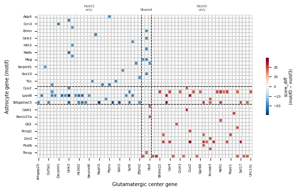
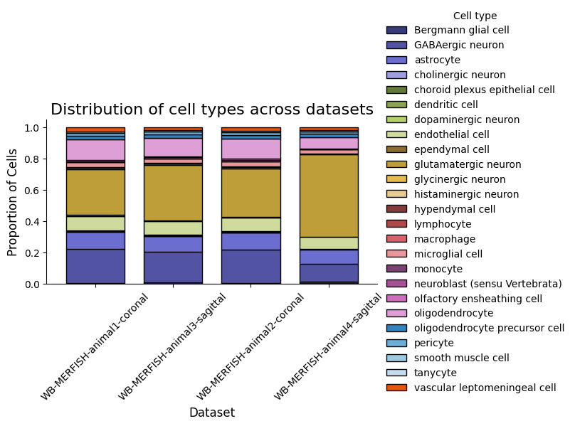
This tutorial demonstrates spatial analysis of a large-scale MERFISH whole-brain atlas (~8.4 million cells across 239 brain sections from 4 animals). We use spatial_query_multi to discover spatial motifs surrounding glutamatergic neurons, examine their regional distribution, perform cross-cell gene-gene covariation analysis, and compare motif-specific covarying gene programs across brain regions.

Dataset: Allen Institute WB-MERFISH adult mouse brain atlas API class: spatial_query_multi

1. Setup

import warnings
warnings.filterwarnings("ignore")

import os
import anndata as ad
import numpy as np
import pandas as pd
import matplotlib.pyplot as plt
import seaborn as sns

from SpatialQuery import spatial_query_multi

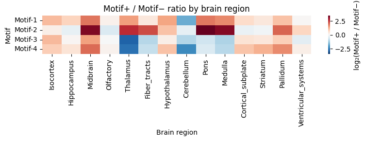
2. Load Data

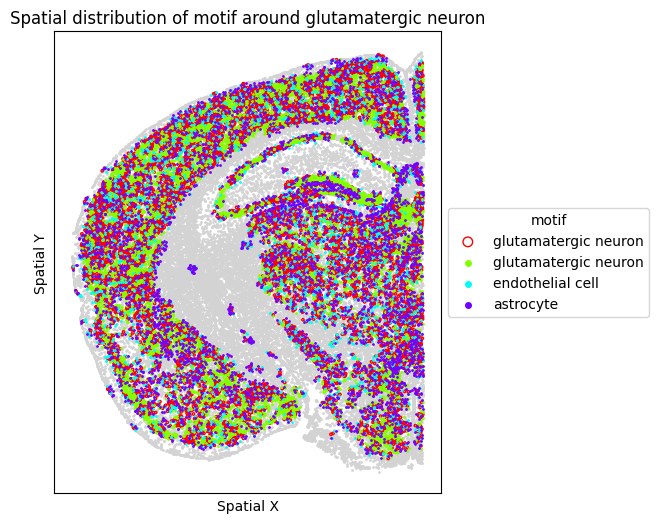
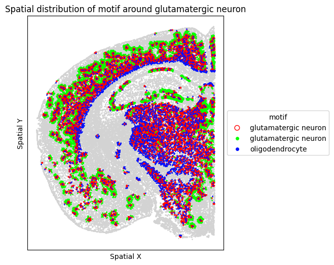
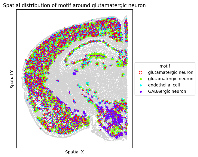
The MERFISH atlas consists of 4 animals (2 coronal, 2 sagittal) with 239 brain sections total.

DATA_DIR = "../data/merfish_mouse_brain"

files = [f for f in os.listdir(DATA_DIR) if f.endswith(".h5ad")]
adatas = [ad.read_h5ad(os.path.join(DATA_DIR, f)) for f in files]
adatas[0]

AnnData object with n_obs × n_vars = 1915592 × 1120
    obs: 'donor_id', 'development_stage_ontology_term_id', 'sex_ontology_term_id', 'self_reported_ethnicity_ontology_term_id', 'disease_ontology_term_id', 'tissue_ontology_term_id', 'cell_type_ontology_term_id', 'assay_ontology_term_id', 'suspension_type', 'cluster_id_transfer', 'subclass_transfer', 'cluster_confidence_score', 'subclass_confidence_score', 'high_quality_transfer', 'major_brain_region', 'ccf_region_name', 'brain_section_label', 'tissue_type', 'is_primary_data', 'cell_type', 'assay', 'disease', 'sex', 'tissue', 'self_reported_ethnicity', 'development_stage', 'observation_joinid'
    var: 'gene_name', 'feature_is_filtered', 'feature_name', 'feature_reference', 'feature_biotype', 'feature_length', 'feature_type'
    uns: 'citation', 'organism', 'organism_ontology_term_id', 'schema_reference', 'schema_version', 'title'
    obsm: 'X_CCF', 'X_spatial_coords', 'X_umap'

# Split each animal into individual brain sections
adatas_fov = []
dataset_names = []
for adata in adatas:
    dataset_name = adata.uns["title"]
    for label in adata.obs["brain_section_label"].unique():
        adatas_fov.append(adata[adata.obs["brain_section_label"] == label].copy())
    dataset_names.extend([dataset_name] * len(adata.obs["brain_section_label"].unique()))

print(f"Total FOVs: {len(adatas_fov)}")
print(f"Total cells: {sum(a.n_obs for a in adatas_fov):,}")

Total FOVs: 239
Total cells: 8,380,288

print(f'Max value: {adata.X.max()}, min value: {adata.X.min()}')

Max value: 6.908754825592041, min value: 0.0

Data is already log-normalized. We skip normalization during initialization (if_lognorm=False).

3. Initialize SpatialQuery Multi

# ---- Configuration: adjust these to match your dataset ----
spatial_key = "X_spatial_coords"
label_key = "cell_type"
feature_name = "gene_name"

spm = spatial_query_multi(
    adatas_fov,
    datasets=dataset_names,
    spatial_key=spatial_key,
    label_key=label_key,
    feature_name=feature_name,
    build_gene_index=False,
    if_lognorm=False,
    if_normalize_spatial_coord=True,
)

Replacing _ with hyphen in WB_MERFISH_animal2_coronal.
Replacing _ with hyphen in WB_MERFISH_animal2_coronal.
Replacing _ with hyphen in WB_MERFISH_animal2_coronal.
Replacing _ with hyphen in WB_MERFISH_animal2_coronal.
Replacing _ with hyphen in WB_MERFISH_animal2_coronal.
Replacing _ with hyphen in WB_MERFISH_animal2_coronal.
Replacing _ with hyphen in WB_MERFISH_animal2_coronal.
Replacing _ with hyphen in WB_MERFISH_animal2_coronal.
Replacing _ with hyphen in WB_MERFISH_animal2_coronal.
Replacing _ with hyphen in WB_MERFISH_animal2_coronal.
... (1183 lines omitted) ...
Scale factor: 0.0843
build_gene_index is False. Using adata.X for gene expression analysis.

valid_ds_names = sorted(set(d.split("_")[0] for d in spm.datasets))
print(valid_ds_names)

['WB-MERFISH-animal1-coronal', 'WB-MERFISH-animal2-coronal', 'WB-MERFISH-animal3-sagittal', 'WB-MERFISH-animal4-sagittal']

4. Cell Type Composition

from matplotlib.colors import ListedColormap
import matplotlib.cm as cm

# Combine tab20b + tab20c for 40 unique colors (needed when >20 cell types)
all_colors = []
for name in ["tab20b", "tab20c"]:
    cmap = cm.get_cmap(name)
    all_colors.extend([cmap(i) for i in range(cmap.N)])

seen = set()
unique_colors = []
for c in all_colors:
    key = tuple(round(v, 4) for v in c)
    if key not in seen:
        seen.add(key)
        unique_colors.append(c)

custom_cmap = ListedColormap(unique_colors, name="tab40")

spm.plot_cell_type_distribution(colormap=custom_cmap)

/var/folders/wl/y90xsxr94l78931lqz6nyvz80000gp/T/ipykernel_31656/3661813038.py:7: MatplotlibDeprecationWarning: The get_cmap function was deprecated in Matplotlib 3.7 and will be removed in 3.11. Use ``matplotlib.colormaps[name]`` or ``matplotlib.colormaps.get_cmap()`` or ``pyplot.get_cmap()`` instead.
  cmap = cm.get_cmap(name)
/var/folders/wl/y90xsxr94l78931lqz6nyvz80000gp/T/ipykernel_31656/3661813038.py:7: MatplotlibDeprecationWarning: The get_cmap function was deprecated in Matplotlib 3.7 and will be removed in 3.11. Use ``matplotlib.colormaps[name]`` or ``matplotlib.colormaps.get_cmap()`` or ``pyplot.get_cmap()`` instead.
  cmap = cm.get_cmap(name)
/Users/sa3520/BWH/spatial query/python/SpatialQuery/spatial_query_multiple_fov.py:1441: MatplotlibDeprecationWarning: The get_cmap function was deprecated in Matplotlib 3.7 and will be removed in 3.11. Use ``matplotlib.colormaps[name]`` or ``matplotlib.colormaps.get_cmap()`` or ``pyplot.get_cmap()`` instead.
  cmap = cm.get_cmap(colormap)

5. Motif Enrichment Analysis

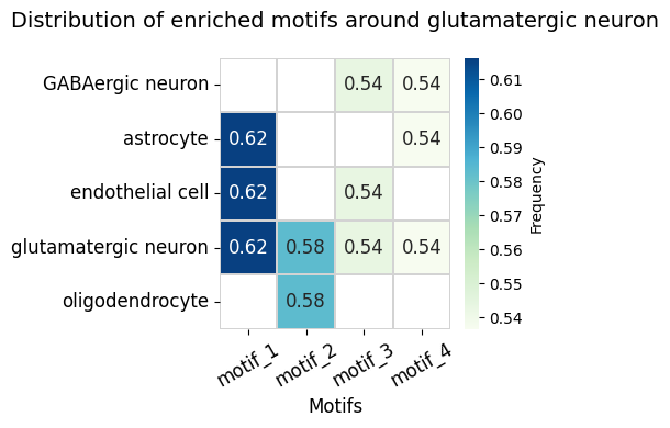
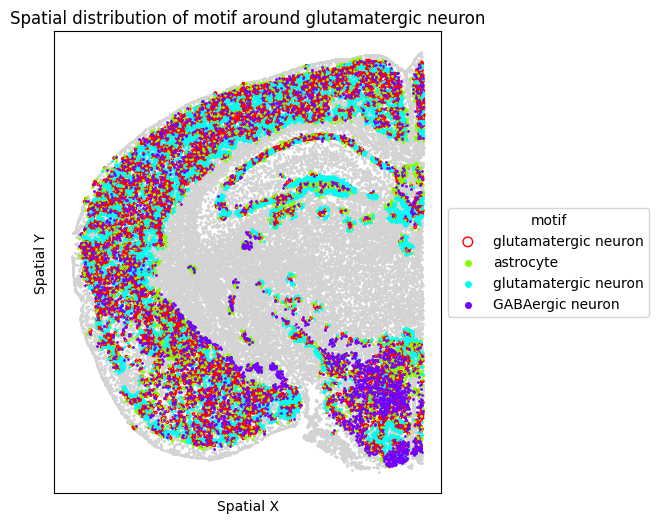
Discover enriched motifs surrounding glutamatergic neurons in coronal sections. We restrict to coronal datasets for consistency across animals.

anchor_ct = 'glutamatergic neuron'
max_dist = 5
min_support = 0.5

coronal_ds = ['WB-MERFISH-animal1-coronal', 'WB-MERFISH-animal2-coronal']

motif_glut_coronal_df, motif_glut_coronal_motif_id, motif_glut_coronal_center_id = spm.motif_enrichment_dist(
    ct=anchor_ct,
    dataset=coronal_ds,
    max_dist=max_dist,
    min_support=min_support,
    return_cellID=True
)

from SpatialQuery.plotting import plot_motif_enrichment_heatmap
plot_motif_enrichment_heatmap(enrich_df=motif_glut_coronal_df,
                              figsize=(5, 4),
                              )

# Collect motif+ / motif- obs for each motif

data_by_motif = {}
for motif_idx in range(len(motif_glut_coronal_df)):
    motifs_list = motif_glut_coronal_df.iloc[motif_idx]['motifs']
    outer_key = str(sorted(motifs_list))
    center_id_dict = motif_glut_coronal_center_id.get(outer_key, {})

    pos_obs_list, neg_obs_list = [], []
    for sp, fov_ds in zip(spm.spatial_queries, spm.datasets):
        if not any(fov_ds.startswith(td) for td in coronal_ds):
            continue
        obs = sp.adata.obs.copy()
        ct_mask = obs[label_key] == anchor_ct
        pos_indices = center_id_dict.get(fov_ds, [])
        if len(pos_indices) > 0:
            pos_mask = np.zeros(len(obs), dtype=bool)
            pos_mask[np.asarray(pos_indices)] = True
            pos_obs_list.append(obs[pos_mask & ct_mask])
            neg_obs_list.append(obs[ct_mask & ~pos_mask])
        else:
            neg_obs_list.append(obs[ct_mask])

    pos_obs = pd.concat(pos_obs_list, ignore_index=True) if pos_obs_list else pd.DataFrame()
    neg_obs = pd.concat(neg_obs_list, ignore_index=True) if neg_obs_list else pd.DataFrame()
    motif_label = '+'.join(sorted([m for m in motifs_list if m != anchor_ct])) or 'Self'
    data_by_motif[motif_idx] = dict(pos_obs=pos_obs, neg_obs=neg_obs, motif_label=motif_label)

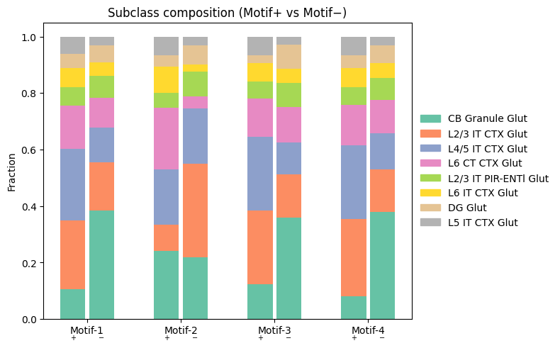
# Subclass composition (motif+ vs motif-) per motif
import matplotlib.patches as mpatches

all_obs = pd.concat(
    [d['pos_obs'] for d in data_by_motif.values()] +
    [d['neg_obs'] for d in data_by_motif.values()],
    ignore_index=True
)
top_subs = all_obs['subclass_transfer'].value_counts().index[:8].tolist()

n_motifs = len(data_by_motif)
bar_w, gap = 0.35, 0.05
x_centers = np.arange(n_motifs) * 1.3
cmap = plt.cm.get_cmap('Set2', len(top_subs))
sub_colors = {s: cmap(i) for i, s in enumerate(top_subs)}

fig, ax = plt.subplots(figsize=(max(6, n_motifs * 2), 5))
for motif_idx, d in data_by_motif.items():
    for obs_df, x_bar in [(d['pos_obs'], x_centers[motif_idx]),
                           (d['neg_obs'], x_centers[motif_idx] + bar_w + gap)]:
        if len(obs_df) == 0:
            continue
        counts = obs_df['subclass_transfer'].value_counts(normalize=True)
        top_fracs = {sub: counts.get(sub, 0.0) for sub in top_subs}
        total_top = sum(top_fracs.values())
        if total_top == 0:
            continue
        bottom = 0.0
        for sub in top_subs:
            frac = top_fracs[sub] / total_top
            ax.bar(x_bar, frac, bar_w, bottom=bottom, color=sub_colors[sub])
            bottom += frac

tick_pos = [x_centers[i] + (bar_w + gap) / 2 for i in range(n_motifs)]
ax.set_xticks(tick_pos)
ax.set_xticklabels([f'Motif-{i+1}' for i in range(n_motifs)])
for i in range(n_motifs):
    ax.text(x_centers[i], -0.05, '+', ha='center', va='top', fontsize=7, transform=ax.get_xaxis_transform())
    ax.text(x_centers[i] + bar_w + gap, -0.05, '−', ha='center', va='top', fontsize=7, transform=ax.get_xaxis_transform())

ax.legend(handles=[mpatches.Patch(color=sub_colors[s], label=s) for s in top_subs],
          loc='center left', bbox_to_anchor=(1, 0.5), frameon=False)
ax.set_ylabel('Fraction')
ax.set_title('Subclass composition (Motif+ vs Motif−)')
plt.tight_layout()

/var/folders/wl/y90xsxr94l78931lqz6nyvz80000gp/T/ipykernel_31656/514646767.py:14: MatplotlibDeprecationWarning: The get_cmap function was deprecated in Matplotlib 3.7 and will be removed in 3.11. Use ``matplotlib.colormaps[name]`` or ``matplotlib.colormaps.get_cmap()`` or ``pyplot.get_cmap()`` instead.
  cmap = plt.cm.get_cmap('Set2', len(top_subs))

# Heatmap: Motif+ / Motif- ratio per brain region
region_order = list(data_by_motif[0]['pos_obs']['major_brain_region'].value_counts().index)

rows = {}
for motif_idx, d in data_by_motif.items():
    pos_region = d['pos_obs']['major_brain_region'].value_counts()
    neg_region = d['neg_obs']['major_brain_region'].value_counts()
    ratio = pd.Series({
        r: pos_region.get(r, 0) / max(neg_region.get(r, 0), 1)
        for r in region_order
    })
    rows[f'Motif-{motif_idx+1}'] = ratio

hm_df = pd.DataFrame(rows, index=region_order).T
log2_df = np.log2(hm_df.clip(lower=1e-6))
abs_max = np.nanmax(np.abs(log2_df.values))

fig, ax = plt.subplots(figsize=(8, max(3, n_motifs * 0.6)))
sns.heatmap(
    log2_df, ax=ax, cmap='RdBu_r',
    vmin=-abs_max, vmax=abs_max, center=0,
    cbar_kws={'label': 'log₂(Motif+ / Motif−)'},
)
ax.set_xticklabels(ax.get_xticklabels(), rotation=90)
ax.set_yticklabels(ax.get_yticklabels(), rotation=0)
ax.set_xlabel('Brain region')
ax.set_ylabel('Motif')
ax.set_title('Motif+ / Motif− ratio by brain region')
plt.tight_layout()

# Visualize motif distribution in a single representative FOV
target_fov = "WB-MERFISH-animal2-coronal_49"
target_sp = [sp for sp in spm.spatial_queries if sp.dataset == target_fov][0]

for m in motif_glut_coronal_df["motifs"]:
    target_sp.plot_motif_celltype(
        ct=anchor_ct,
        motif=m,
        max_dist=max_dist,
        figsize=(5, 6),
    )

6. Cross-cell Gene-Gene Covariation

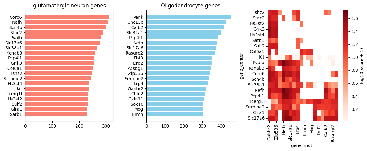
Identify gene pairs with spatially-specific cross-cell correlation between glutamatergic neurons and their motif neighbors.

print(f"Anchor: {anchor_ct}, max_dist: {max_dist}")
print(f"Coronal datasets: {coronal_ds}")

Anchor: glutamatergic neuron, max_dist: 5
Coronal datasets: ['WB-MERFISH-animal1-coronal', 'WB-MERFISH-animal2-coronal']

motif2 = ['oligodendrocyte', 'glutamatergic neuron']
covarying_genes_m2 = spm.compute_gene_gene_correlation_by_type(
    ct=anchor_ct,
    motif=motif2,
    dataset=coronal_ds,
    max_dist=max_dist,
)

Computing covarying genes using expression data ...
Only one non-center cell type in motif: ['oligodendrocyte']. Using compute_gene_gene_correlation method.
No genes specified. Using union of genes across all selected FOVs ...
Gene coverage: 1120 genes in all FOVs, 1120 genes total (union)
Analyzing 1120 genes across 213 FOVs

================================================================================
Step 1: Computing and accumulating statistics across FOVs
================================================================================

... (1523 lines omitted) ...
Total gene pairs analyzed: 1254400
Significant pairs: 151030

covarying_genes_m2 = covarying_genes_m2[covarying_genes_m2['if_significant']]
covarying_genes_m2

	gene_center	gene_motif	corr_neighbor	corr_non_neighbor	p_value_test1	delta_corr_test1	corr_center_no_motif	p_value_test2	delta_corr_test2	combined_score	adj-pval-test1	adj-pval-test2	if_significant	cell_type
0	Prkcd	Prkcd	0.483658	-0.025477	0.0	0.509135	0.066700	0.0	0.416958	133.383376	0.0	0.0	True	oligodendrocyte
1	Grik3	Slc17a7	0.200625	-0.046645	0.0	0.247271	-0.169207	0.0	0.369833	99.919199	0.0	0.0	True	oligodendrocyte
2	Tnnt1	Prkcd	0.318601	-0.015084	0.0	0.333685	0.008595	0.0	0.310006	95.132929	0.0	0.0	True	oligodendrocyte
3	Grid2ip	Prkcd	0.353341	-0.021876	0.0	0.375217	0.065240	0.0	0.288100	94.270543	0.0	0.0	True	oligodendrocyte
4	Rgs16	Prkcd	0.316480	-0.020070	0.0	0.336550	0.023593	0.0	0.292886	91.795601	0.0	0.0	True	oligodendrocyte
...	...	...	...	...	...	...	...	...	...	...	...	...	...	...
1254395	Gucy1a1	Slc17a7	-0.098372	0.052502	0.0	-0.150874	0.172281	0.0	-0.270654	-70.415942	0.0	0.0	True	oligodendrocyte
1254396	Cux2	Slc17a7	-0.146541	0.030721	0.0	-0.177261	0.150265	0.0	-0.296806	-78.282743	0.0	0.0	True	oligodendrocyte
1254397	Otof	Slc17a7	-0.153165	0.065437	0.0	-0.218603	0.149220	0.0	-0.302385	-83.175139	0.0	0.0	True	oligodendrocyte
1254398	Calb1	Slc17a7	-0.166215	0.052068	0.0	-0.218283	0.136621	0.0	-0.302836	-83.241135	0.0	0.0	True	oligodendrocyte
1254399	Syt17	Slc17a7	-0.115302	0.056794	0.0	-0.172096	0.233440	0.0	-0.348742	-88.724367	0.0	0.0	True	oligodendrocyte

151030 rows × 14 columns

# Covarying gene pairs for motif2 (oligodendrocyte)
oligo_pos = covarying_genes_m2[covarying_genes_m2['cell_type'] == 'oligodendrocyte'].copy()
oligo_pos = oligo_pos[oligo_pos['combined_score'] > 0]

top_gene_center = pd.DataFrame(oligo_pos['gene_center'].value_counts().head(20))[::-1]
top_gene_motif = pd.DataFrame(oligo_pos['gene_motif'].value_counts().head(20))[::-1]

fig, axs = plt.subplots(1, 3, figsize=(12, 5))

axs[0].barh(top_gene_center.index.tolist(), top_gene_center['count'].tolist(), color='salmon')
axs[0].set_title(f'{anchor_ct} genes')

axs[1].barh(top_gene_motif.index.tolist(), top_gene_motif['count'].tolist(), color='skyblue')
axs[1].set_title('Oligodendrocyte genes')

# Heatmap of top50 gene pairs
from scipy.cluster.hierarchy import linkage, dendrogram
from scipy.spatial.distance import pdist

top20_center = oligo_pos['gene_center'].value_counts().head(20).index.tolist()
top20_motif = oligo_pos['gene_motif'].value_counts().head(20).index.tolist()
sub = oligo_pos[oligo_pos['gene_center'].isin(top20_center) & oligo_pos['gene_motif'].isin(top20_motif)]

pivot = sub.pivot_table(index='gene_center', columns='gene_motif', values='combined_score', fill_value=0)
mask = (pivot == 0)
data = np.log10(pivot + 1)

row_order = dendrogram(linkage(pdist(data), method='average'), no_plot=True)['leaves']
col_order = dendrogram(linkage(pdist(data.T), method='average'), no_plot=True)['leaves']

sns.heatmap(
    data.iloc[row_order, col_order],
    mask=mask.iloc[row_order, col_order],
    cmap='Reds',
    cbar_kws={'label': 'log10(score + 1)'},
    ax=axs[2],
)

plt.tight_layout()

7. Regional Stratification: Isocortex Analysis

Since glutamatergic neurons are most abundant in the Isocortex, we construct a subset containing only Isocortex cells and repeat the covariation analysis to examine whether motif-specific gene programs are preserved in a single brain region.

# Subset to Isocortex cells from coronal sections
adatas_coronal_isocortex = []
dataset_names_coronal_isocortex = []

adatas_coronal = [adatas_fov[i] for i in range(len(adatas_fov)) if "coronal" in adatas_fov[i].uns["title"]]

for adata in adatas_coronal:
    sub_data = adata[adata.obs["major_brain_region"] == "Isocortex"].copy()
    adatas_coronal_isocortex.append(sub_data)
    dataset_names_coronal_isocortex.append(adata.uns["title"])

print(f"Isocortex FOVs: {len(adatas_coronal_isocortex)}")
print(f"Isocortex cells: {sum(a.n_obs for a in adatas_coronal_isocortex):,}")

Isocortex FOVs: 213
Isocortex cells: 1,337,180

spm_coronal_isocortex = spatial_query_multi(
    adatas=adatas_coronal_isocortex,
    datasets=dataset_names_coronal_isocortex,
    spatial_key=spatial_key,
    label_key=label_key,
    build_gene_index=False,
    feature_name=feature_name,
    if_lognorm=False,
    if_normalize_spatial_coord=True
)

Replacing _ with hyphen in WB_MERFISH_animal2_coronal.
Replacing _ with hyphen in WB_MERFISH_animal2_coronal.
Replacing _ with hyphen in WB_MERFISH_animal2_coronal.
Replacing _ with hyphen in WB_MERFISH_animal2_coronal.
Replacing _ with hyphen in WB_MERFISH_animal2_coronal.
Replacing _ with hyphen in WB_MERFISH_animal2_coronal.
Replacing _ with hyphen in WB_MERFISH_animal2_coronal.
Replacing _ with hyphen in WB_MERFISH_animal2_coronal.
Replacing _ with hyphen in WB_MERFISH_animal2_coronal.
Replacing _ with hyphen in WB_MERFISH_animal2_coronal.
... (1053 lines omitted) ...
Scale factor: 0.0881
build_gene_index is False. Using adata.X for gene expression analysis.

motif0 = motif_glut_coronal_df['motifs'].iloc[0]

covarying_isocortex_motif0 = spm_coronal_isocortex.compute_gene_gene_correlation_by_type(
    ct=anchor_ct,
    motif=motif0,
    dataset=coronal_ds,
    max_dist=max_dist,
)

Computing covarying genes using expression data ...
Analyzing 2 non-center cell types in motif: ['astrocyte', 'endothelial cell']
================================================================================
Selected 213 FOVs for analysis
No genes specified. Using union of genes across all selected FOVs ...
Gene coverage: 1120 genes in all FOVs, 1120 genes total (union)
Analyzing 1120 genes across 213 FOVs

================================================================================
Step 1: Computing Correlation-3 (Center without motif vs Neighbors)
... (938 lines omitted) ...

Results prepared and sorted

motif3 = motif_glut_coronal_df['motifs'].iloc[3]

covarying_isocortex_motif3 = spm_coronal_isocortex.compute_gene_gene_correlation_by_type(
    ct=anchor_ct,
    motif=motif3,
    dataset=coronal_ds,
    max_dist=max_dist,
)

Computing covarying genes using expression data ...
Analyzing 2 non-center cell types in motif: ['GABAergic neuron', 'astrocyte']
================================================================================
Selected 213 FOVs for analysis
No genes specified. Using union of genes across all selected FOVs ...
Gene coverage: 1120 genes in all FOVs, 1120 genes total (union)
Analyzing 1120 genes across 213 FOVs

================================================================================
Step 1: Computing Correlation-3 (Center without motif vs Neighbors)
... (938 lines omitted) ...

Results prepared and sorted

covarying_isocortex_motif3_astro = covarying_isocortex_motif3[covarying_isocortex_motif3['if_significant']]
covarying_isocortex_motif3_astro = covarying_isocortex_motif3_astro[covarying_isocortex_motif3_astro['cell_type'] == 'astrocyte']

covarying_isocortex_motif0_astro = covarying_isocortex_motif0[covarying_isocortex_motif0['if_significant']]
covarying_isocortex_motif0_astro = covarying_isocortex_motif0_astro[covarying_isocortex_motif0_astro['cell_type'] == 'astrocyte']

rank_genes_glut_astro_isocortex = spm_coronal_isocortex.test_score_difference(
    result_A=covarying_isocortex_motif0_astro,
    result_B=covarying_isocortex_motif3_astro,
    percentile_threshold=99
)

Significant pairs in A: 6652
Significant pairs in B: 7929
Pairs that are significant in at least one group: 9350
Time to compute percentiles: 0.11 seconds.

============================================================
Score Difference Test Results
============================================================
Total pairs tested: 5231
Outlier pairs (percentile > 99 or < 1): 105
... (4 lines omitted) ...
Mean score difference: 0.199
Std score difference: 5.155

df_plot = rank_genes_glut_astro_isocortex[rank_genes_glut_astro_isocortex['outlier_direction'] != 'not_outlier'].copy()

m0 = df_plot[df_plot['outlier_direction'] == 'higher_in_A'].nlargest(100, 'score_diff')
m3 = df_plot[df_plot['outlier_direction'] == 'lower_in_A'].nsmallest(100, 'score_diff')
df_plot = pd.concat([m0, m3])

center_shared  = sorted(set(m0['gene_center']) & set(m3['gene_center']))
center_m0_only = sorted(set(m0['gene_center']) - set(m3['gene_center']))
center_m3_only = sorted(set(m3['gene_center']) - set(m0['gene_center']))
center_genes   = center_m3_only + center_shared + center_m0_only

motif_shared   = sorted(set(m0['gene_motif']) & set(m3['gene_motif']))
motif_m0_only  = sorted(set(m0['gene_motif']) - set(m3['gene_motif']))
motif_m3_only  = sorted(set(m3['gene_motif']) - set(m0['gene_motif']))
motif_genes    = motif_m3_only + motif_shared + motif_m0_only

n_row = len(center_genes)
n_col = len(motif_genes)
row_idx = {g: i for i, g in enumerate(center_genes)}
col_idx = {g: i for i, g in enumerate(motif_genes)}

mat = np.full((n_row, n_col), np.nan)
for _, row in df_plot.iterrows():
    mat[row_idx[row['gene_center']], col_idx[row['gene_motif']]] = row['score_diff']

vmax = np.nanmax(np.abs(mat))
mat_df = pd.DataFrame(mat, index=center_genes, columns=motif_genes)

mat_df_T = mat_df.T  # rows = astrocyte genes, cols = glut genes

fig, ax = plt.subplots(figsize=(max(4, n_row * 0.1), max(3, n_col * 0.1)))

sns.heatmap(
    mat_df_T,
    cmap='RdBu_r',
    center=0,
    vmin=-vmax, vmax=vmax,
    linewidths=0.01,
    linecolor='lightgrey',
    mask=np.isnan(mat.T),
    cbar_kws={'label': 'score_diff\n(motif0 − motif3)', 'shrink': 0.4},
    ax=ax,
)

cbar = ax.collections[0].colorbar
cbar.ax.tick_params(labelsize=5)
cbar.set_label('score_diff\n(motif0 − motif3)', fontsize=6)

# Dividing lines — seaborn heatmap: col x goes 0..n_col, row y goes 0..n_row
n_m3_only_col = len(motif_m3_only)
n_shared_col  = len(motif_shared)
n_m3_only_row = len(center_m3_only)
n_shared_row  = len(center_shared)

# After transpose: rows = motif genes, cols = center genes
# Dashed lines: column boundaries from original row splits, row boundaries from col splits
for x in [n_m3_only_row, n_m3_only_row + n_shared_row]:
    ax.axvline(x, color='black', linewidth=0.8, linestyle='--')
for y in [n_m3_only_col, n_m3_only_col + n_shared_col]:
    ax.axhline(y, color='black', linewidth=0.8, linestyle='--')

ax.set_xlabel('Glutamatergic center gene', fontsize=7)
ax.set_ylabel('Astrocyte gene (motif)', fontsize=7)
ax.tick_params(axis='x', labelsize=5)
ax.tick_params(axis='y', labelsize=5)

# Region annotations: columns are center genes (motif3-only | shared | motif0-only)
ax.text(n_m3_only_row / 2,                           -1.2, 'Motif3\nonly', ha='center', fontsize=5, color='#555')
ax.text(n_m3_only_row + n_shared_row / 2,            -1.2, 'Shared',       ha='center', fontsize=5, color='#333')
ax.text(n_m3_only_row + n_shared_row + len(center_m0_only) / 2, -1.2, 'Motif0\nonly', ha='center', fontsize=5, color='#555')

plt.tight_layout()
plt.show()