Tutorial 1: Spatial Analysis of a Single Field of View

This tutorial demonstrates the core SpatialQuery workflow on a single spatial transcriptomics dataset. We use a seqFISH mouse organogenesis (E8.5) embryo section containing 17,806 cells and 351 genes. The analysis covers motif enrichment discovery, spatial visualization, differential expression between motif-positive and motif-negative anchor cells, and cross-cell gene-gene covariation analysis.

API class: spatial_query

1. Setup

import warnings
warnings.filterwarnings("ignore")

import anndata as ad
import numpy as np
import pandas as pd
import matplotlib.pyplot as plt
import seaborn as sns

from SpatialQuery import spatial_query

2. Load Data & Initialize SpatialQuery

DATA_DIR = "../data/mouse_organogenesis"

adata = ad.read_h5ad(f"{DATA_DIR}/embryo1.h5ad")
adata

AnnData object with n_obs × n_vars = 17806 × 351
    obs: 'embryo', 'pos', 'z', 'x_global', 'y_global', 'x_global_affine', 'y_global_affine', 'embryo_pos', 'embryo_pos_z', 'Area', 'UMAP1', 'UMAP2', 'celltype_mapped_refined', 'segmentation_vertices_x_global_affine', 'segmentation_vertices_y_global_affine'
    var: 'gene'
    uns: 'celltype_mapped_refined_colors'
    obsm: 'X_spatial', 'X_umap'

# ---- Configuration: adjust these to match your dataset ----
spatial_key = "X_spatial"
label_key = "celltype_mapped_refined"
feature_name = "gene"
dataset_name = "mouse_embryo1"

sp = spatial_query(
    adata=adata,
    dataset=dataset_name,
    spatial_key=spatial_key,
    label_key=label_key,
    feature_name=feature_name,
    build_gene_index=False,       # use adata.X directly for gene expression
    if_lognorm=True,              # log-normalize raw counts
    if_normalize_spatial_coord=True,
)

Auto-normalizing spatial coordinates: mean nearest neighbor distance = 1.0
Scale factor: 51.7200
build_gene_index is False. Using adata.X for gene expression analysis.
Log normalizing the expression data... If data is already log normalized, please set if_lognorm to False.

3. Visualize the Field of View

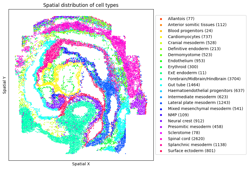
sp.plot_fov(min_cells_label=0, figsize=(8, 6))

4. Motif Enrichment Across Cell Types and Radii

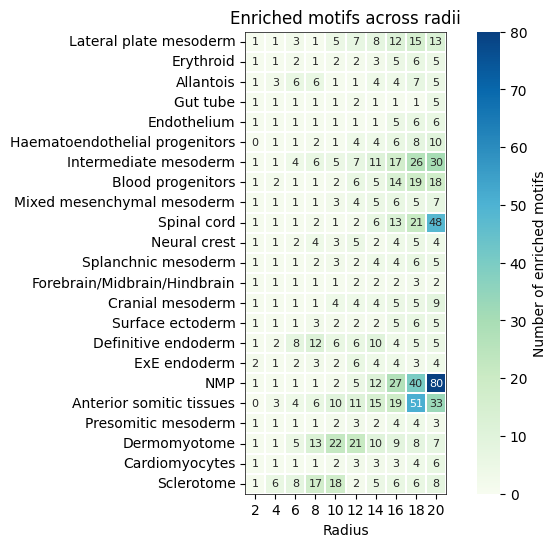
A spatial motif is a recurring combination of cell types found in the neighborhood of an anchor cell type. Here we scan all cell types as anchors across a range of radii to get an overview of spatial organization complexity.

radius_range = list(range(2, 21, 2))
unique_cts = sp.labels.unique().tolist()

enrich_radius_ct = dict()

for ct in unique_cts:
    enrich_radius_ct[ct] = []

    for r in radius_range:
        enrich_tmp = sp.motif_enrichment_dist(
            ct=ct,
            max_dist=r,
            min_support=0.5,
        )
        enrich_tmp = enrich_tmp[enrich_tmp['if_significant']]
        enrich_radius_ct[ct].append(enrich_tmp.shape[0])

enrich_radius_ct_df = pd.DataFrame(enrich_radius_ct, index=radius_range)


fig, ax = plt.subplots(figsize=(8, 6))
sns.heatmap(enrich_radius_ct_df.T,
            cmap='GnBu',
            linewidths=0.1,
            square=True, annot=True, fmt='g',
            annot_kws={'fontsize': 8}, ax=ax, linecolor='white',
            cbar_kws={'label': 'Number of enriched motifs'}
            )
for spine_name, spine in ax.spines.items():
    spine.set_visible(True)
    spine.set_color('black')
    spine.set_linewidth(0.5)
plt.xlabel('Radius')
plt.xticks(rotation=0)
plt.title('Enriched motifs across radii')

Text(0.5, 1.0, 'Enriched motifs across radii')

5. Targeted Motif Enrichment

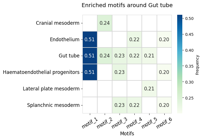
We select Gut tube as the anchor cell type and discover which cell type combinations are significantly enriched in its neighborhood within a radius of 8 (normalized units).

anchor_ct = 'Gut tube'
max_dist = 8
min_support = 0.2

enrich = sp.motif_enrichment_dist(
    ct=anchor_ct,
    max_dist=max_dist,
    min_support=min_support
)

enrich

	center	motifs	n_center_motif	n_center	n_motif	expectation	p-values	adj-pval	if_significant
0	Gut tube	[Endothelium, Gut tube, Haematoendothelial pro...	748	1464	2439	200.533303	1.260625e-290	7.563750e-290	True
1	Gut tube	[Cranial mesoderm, Gut tube]	357	1464	1282	105.405369	4.065308e-107	1.219592e-106	True
2	Gut tube	[Endothelium, Gut tube, Splanchnic mesoderm]	320	1464	1188	97.676738	7.788483e-91	1.557697e-90	True
3	Gut tube	[Gut tube, Haematoendothelial progenitors, Spl...	332	1464	1433	117.820510	1.252217e-75	1.878326e-75	True
4	Gut tube	[Gut tube, Lateral plate mesoderm]	312	1464	1595	131.140065	1.212101e-52	1.454521e-52	True
5	Gut tube	[Endothelium, Haematoendothelial progenitors, ...	293	1464	2863	235.394361	1.308209e-05	1.308209e-05	True

sp.plot_motif_enrichment_heatmap(
    enrich_df=enrich,
    figsize=(7, 5),
    title='Enriched motifs around Gut tube',
)

6. Motif Enrichment Across Radii

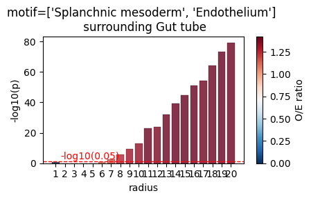
For a specific motif of interest, we examine how enrichment significance and observed/expected ratio change across radii 1–20.

p_vals = []
oe_ratio = []
ct = 'Gut tube'
motif = ['Splanchnic mesoderm', 'Endothelium']
radius_list = range(1, 21)

for i in radius_list:
    tt = sp.motif_enrichment_dist(
        ct=ct,
        motifs=motif,
        max_dist=i
    )
    p_vals.append(tt['p-values'][0])
    oe_ratio.append(tt['n_center_motif'][0]/tt['expectation'][0])

p_vals_df = pd.DataFrame({
    'radius': radius_list,
    '-log_pvals': -np.log10(p_vals),
    'O/E ratio': oe_ratio
})

fig, ax = plt.subplots(figsize=(4.5, 3))

cmap = plt.get_cmap('RdBu_r')
oe = p_vals_df['O/E ratio']
scaled = (oe - oe.min()) / (oe.max() - oe.min())
colors = [cmap(v) for v in scaled]

bars = ax.bar(p_vals_df['radius'].astype(str),
              p_vals_df['-log_pvals'],
              color=colors, edgecolor='black', alpha=0.8, linewidth=0.25)

sm = plt.cm.ScalarMappable(cmap=cmap)
sm.set_clim(oe.min(), oe.max())
plt.colorbar(sm, ax=ax, label='O/E ratio')

thr = -np.log10(0.05)
ax.axhline(thr, color='red', linestyle='--', linewidth=1)
ax.text(0.5, thr + 0.05, '-log10(0.05)', color='red', fontsize=10, va='bottom')

ax.set_ylabel('-log10(p)')
ax.set_xlabel('radius')
ax.set_title(f'motif={motif} \n surrounding {ct}')
plt.tight_layout()
plt.show()

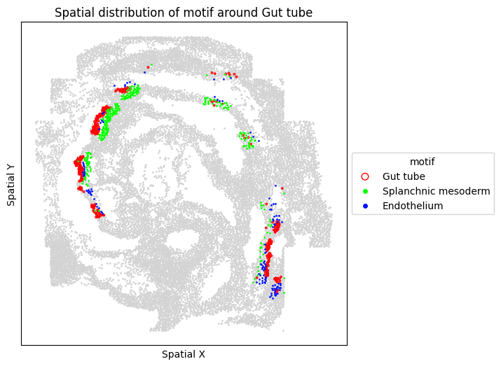
7. Spatial Visualization of Motif

Visualize the spatial distribution of motif-positive anchor cells and their associated neighbor cells.

motif = ["Splanchnic mesoderm", "Endothelium"]

sp.plot_motif_celltype(
    ct=anchor_ct,
    motif=motif,
    max_dist=max_dist,
    figsize=(6, 6),
)

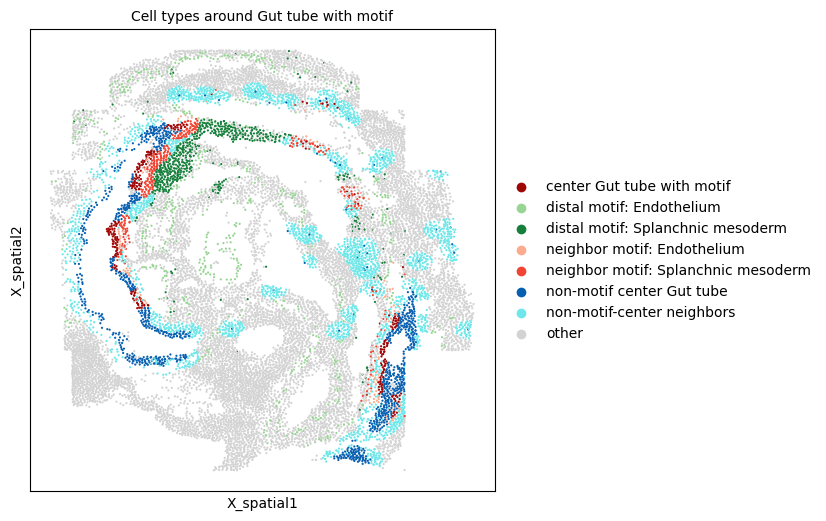
Alternatively, visualize motif-positive vs motif-negative anchor cells alongside motif-associated neighbor cells.

ids = sp.get_anchor_motif_cell_ids(
    ct=anchor_ct,
    motif=motif,
    max_dist=max_dist
)

sp.plot_all_center_motif(
    ct=anchor_ct,
    ids=ids,
)

8. Differential Expression: Motif+ vs Motif− Anchor Cells

Compare gene expression between anchor cells that participate in the motif (motif+) and those that do not (motif−). First, retrieve the cell IDs of motif-positive anchors, then run a t-test across all genes.

motif_enrich = sp.motif_enrichment_dist(
    ct=anchor_ct,
    motifs=motif,
    max_dist=max_dist,
    return_cellID=True
)
motif_enrich

	center	motifs	n_center_motif	n_center	n_motif	expectation	p-values	neighbor_id	center_id	if_significant
0	Gut tube	[Endothelium, Splanchnic mesoderm]	322	1464	3117	256.278109	0.000002	[6151, 6163, 6168, 6182, 6188, 14381, 6199, 62...	[529, 536, 537, 547, 550, 4493, 4611, 4613, 46...	True

center_id = motif_enrich['center_id'][0]
all_center_id = np.where(sp.labels == anchor_ct)[0]
non_center_id = np.setdiff1d(all_center_id, center_id)

de_genes = sp.de_genes(
    ind_group1=center_id,
    ind_group2=non_center_id,
    min_fraction=0.05,
    method='t-test',
    alpha=0.05
)

Testing 351 genes ...

de_genes

	gene	proportion_1	proportion_2	abs_difference	log2fc	p_value	adj-pval	de_in
0	Dkk1	0.111801	0.243433	0.131631	-1.586187	8.074493e-14	1.778115e-11	group2
1	Wnt5a	0.319876	0.472855	0.152979	-1.045780	1.013171e-13	1.778115e-11	group2
2	Osr1	0.652174	0.464974	0.187200	0.943958	2.715462e-12	3.177090e-10	group1
3	T	0.161491	0.260946	0.099455	-1.527118	6.675586e-12	5.857827e-10	group2
4	Meis1	0.503106	0.345009	0.158097	0.959926	1.492688e-09	1.047867e-07	group1
...	...	...	...	...	...	...	...	...
75	Ldhb	0.521739	0.443082	0.078657	0.346249	8.586833e-03	3.965761e-02	group1
76	Pou5f1	0.074534	0.132224	0.057690	-0.778253	8.711626e-03	3.971144e-02	group2
77	Slc4a1	0.071429	0.138354	0.066925	-0.749696	9.692000e-03	4.361400e-02	group2
78	Setd1a	0.723602	0.685639	0.037963	0.261399	1.023892e-02	4.549189e-02	group1
79	Sall3	0.217391	0.292469	0.075078	-0.474529	1.071077e-02	4.699352e-02	group2

80 rows × 8 columns

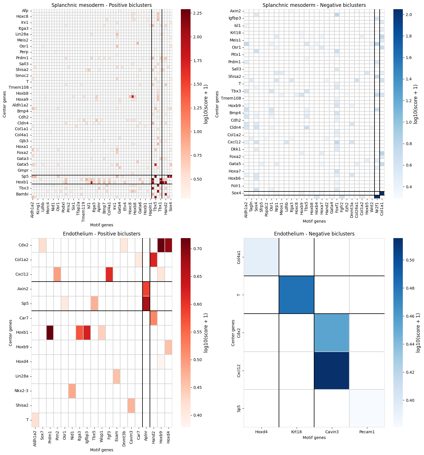
9. Cross-cell Gene-Gene Covariation

Identify gene pairs where one gene is expressed in the anchor cell and the other in a neighboring motif cell, and their expression levels are significantly correlated — specifically in the spatial context of this motif.

covarying_genes_by_type = sp.compute_gene_gene_correlation_by_type(
    ct=anchor_ct,
    motif=motif,
    max_dist=max_dist,
)

covarying_genes_by_type = covarying_genes_by_type[covarying_genes_by_type['if_significant']]

Computing covarying genes using expression data...
Analyzing 2 non-center cell types in motif: ['Splanchnic mesoderm', 'Endothelium']
================================================================================
After filtering (min_nonzero=10): 351 genes

================================================================================
Computing Correlation-3: Center without motif vs Neighbors
================================================================================
Unique center cells: 1106
Unique neighbor cells: 2851
... (55 lines omitted) ...

Results prepared and sorted

covarying_genes_by_type

	cell_type	gene_center	gene_motif	corr_neighbor	corr_non_neighbor	p_value_test1	delta_corr_test1	corr_center_no_motif	p_value_test2	delta_corr_test2	combined_score	q_value_test1	q_value_test2	reject_test1_fdr	reject_test2_fdr	abs_combined_score	if_significant
0	Splanchnic mesoderm	Sp5	Tbx5	0.696998	-0.004279	0.000000e+00	0.701277	0.076782	0.000000	0.620216	193.360220	0.000000	0.000000	True	True	193.360220	True
1	Splanchnic mesoderm	Nkx2-3	Tagln	0.576550	-0.006229	0.000000e+00	0.582779	-0.047309	0.000000	0.623860	183.460727	0.000000	0.000000	True	True	183.460727	True
2	Splanchnic mesoderm	Hoxb1	Tbx1	0.606402	-0.030189	0.000000e+00	0.636591	0.063244	0.000000	0.543158	171.356423	0.000000	0.000000	True	True	171.356423	True
3	Splanchnic mesoderm	Sp5	Wnt2	0.596063	0.000067	0.000000e+00	0.595996	0.150484	0.000000	0.445579	147.211285	0.000000	0.000000	True	True	147.211285	True
4	Splanchnic mesoderm	Tbx3	Tagln	0.395296	-0.000074	1.286408e-07	0.395370	-0.165390	0.000000	0.560686	118.561425	0.000158	0.000000	True	True	118.561425	True
...	...	...	...	...	...	...	...	...	...	...	...	...	...	...	...	...	...
771	Splanchnic mesoderm	Hoxb9	Meox1	0.289525	0.000234	1.691007e-04	0.289292	0.045858	0.000073	0.243667	1.032991	0.047793	0.025269	True	True	1.032991	True
772	Splanchnic mesoderm	Gata3	Hapln1	0.289761	-0.004068	1.341177e-04	0.293829	0.047934	0.000082	0.241827	1.032853	0.040498	0.027817	True	True	1.032853	True
848	Splanchnic mesoderm	Podxl	Ezh2	-0.292342	0.004740	1.120631e-04	-0.297082	-0.060807	0.000157	-0.231535	-0.968453	0.035351	0.045551	True	True	0.968453	True
852	Splanchnic mesoderm	Col1a2	Msx2	0.302228	0.004728	1.043428e-04	0.297501	0.072039	0.000162	0.230189	0.966198	0.033499	0.046536	True	True	0.966198	True
896	Splanchnic mesoderm	Lin28a	Hoxb8	-0.287547	0.004758	1.464706e-04	-0.292305	-0.057600	0.000179	-0.229946	-0.939486	0.043134	0.049649	True	True	0.939486	True

411 rows × 17 columns

covarying_genes_module = sp.plot_gene_pair_heatmap(
    gene_pair_df=covarying_genes_by_type,
    figsize=(15, 8)
)

covarying_genes_module

	gene_center	gene_motif	combined_score	cluster_type	cluster_row	cluster_col	cell_type
0	Afp	Gata4	1.131970	positive	0	0	Splanchnic mesoderm
1	Akr1c19	Gata4	1.507798	positive	0	0	Splanchnic mesoderm
2	Aldh1a2	Tbx5	1.037975	positive	0	1	Splanchnic mesoderm
3	Axin2	Aldh1a2	4.586966	positive	0	0	Splanchnic mesoderm
4	Axin2	Foxf1	1.081744	positive	0	0	Splanchnic mesoderm
...	...	...	...	...	...	...	...
406	Cdx2	Cavin3	-1.846188	negative	2	2	Endothelium
407	Col4a1	Hoxd4	-1.471384	negative	0	0	Endothelium
408	Cxcl12	Cavin3	-2.278150	negative	2	2	Endothelium
409	Sp5	Pecam1	-1.402200	negative	2	2	Endothelium
410	T	Krt18	-2.032839	negative	1	1	Endothelium

411 rows × 7 columns