Tutorial 3: Spatial Proteomics Analysis of Tumor Microenvironment

This tutorial demonstrates multi-condition spatial analysis using CODEX spatial proteomics data from colorectal cancer (CRC) tissue. The dataset contains two immune subtypes — CLR (Crohn’s-Like Reaction) and DII (Diffuse Inflammatory Infiltration) — each with multiple fields of view (FOVs).

We use spatial_query_multi to compare spatial motif patterns between conditions, perform differential motif analysis, and examine hypothesis-driven motifs such as tertiary lymphoid structures (TLS) and immunosuppressive niches.

API class: spatial_query_multi

1. Setup

import warnings
warnings.filterwarnings("ignore")

import os
import anndata as ad
import numpy as np
import pandas as pd
import matplotlib.pyplot as plt
import seaborn as sns

from SpatialQuery import spatial_query_multi

2. Load & Preprocess Data

The CODEX data contains raw protein intensities. We assign disease state labels, apply z-score normalization, and split by FOV for multi-dataset analysis.

# ---- Configuration: adjust these to match your dataset ----
DATA_DIR = "../data/codex_cancer"

adata = ad.read_h5ad(f"{DATA_DIR}/codex_data.h5ad")

adata

AnnData object with n_obs × n_vars = 258385 × 56
    obs: 'CellID', 'ClusterID', 'EventID', 'File Name', 'Region', 'TMA_AB', 'TMA_12', 'Index in File', 'groups', 'patients', 'spots', 'cell_id', 'size:size', 'HOECHST1_Cyc_1_ch_1', 'DRAQ5_Cyc_23_ch_4', 'Profile_Homogeneity:Fiter1', 'ClusterSize', 'ClusterName', 'neighborhood10', 'CD4+ICOS+', 'CD4+Ki67+', 'CD4+PD-1+', 'CD68+CD163+ICOS+', 'CD68+CD163+Ki67+', 'CD68+CD163+PD-1+', 'CD68+ICOS+', 'CD68+Ki67+', 'CD68+PD-1+', 'CD8+ICOS+', 'CD8+Ki67+', 'CD8+PD-1+', 'Treg-ICOS+', 'Treg-Ki67+', 'Treg-PD-1+', 'neighborhood number final', 'neighborhood name'
    var: 'marker_name', 'full_name', 'cell_type_annotation', 'cycle', 'channel'
    uns: 'data_source', 'groups_mapping', 'n_markers', 'technology'
    obsm: 'X_spatial_global', 'X_spatial_tile'

# Assign immune subtype labels based on group ID
adata.obs["state"] = "CLR"
adata.obs["state"][adata.obs["groups"] == 2] = "DII"

print(f"Max value: {adata.X.max()}")

Max value: 54776.6953125

# Feature-wise z-score normalization for protein expression
adata.X = (adata.X - adata.X.mean(axis=0)) / adata.X.std(axis=0)

# Split data by FOV and immune subtype
fov_key = "File Name"

clr_data = adata[adata.obs["state"] == "CLR"]
dii_data = adata[adata.obs["state"] == "DII"]

clr_datas = [clr_data[clr_data.obs[fov_key] == f] for f in clr_data.obs[fov_key].unique()]
dii_datas = [dii_data[dii_data.obs[fov_key] == f] for f in dii_data.obs[fov_key].unique()]

ds_names = ["CLR"] * len(clr_datas) + ["DII"] * len(dii_datas)
adata_fovs = clr_datas + dii_datas

3. Initialize SpatialQuery Multi

Since this is protein data is z-score normalized, we set if_lognorm=False.

# ---- Configuration: adjust these to match your dataset ----
spatial_key = "X_spatial_tile"
label_key = "ClusterName"
feature_name = "marker_name"

spm = spatial_query_multi(
    adatas=adata_fovs,
    datasets=ds_names,
    spatial_key=spatial_key,
    label_key=label_key,
    feature_name=feature_name,
    build_gene_index=False,
    if_lognorm=False,              # data is z-score normalized beforehand
    if_normalize_spatial_coord=True,
)

Auto-normalizing spatial coordinates: mean nearest neighbor distance = 1.0
Scale factor: 0.0448
build_gene_index is False. Using adata.X for gene expression analysis.

Auto-normalizing spatial coordinates: mean nearest neighbor distance = 1.0
Scale factor: 0.0311
build_gene_index is False. Using adata.X for gene expression analysis.

Auto-normalizing spatial coordinates: mean nearest neighbor distance = 1.0
... (548 lines omitted) ...
Scale factor: 0.0421
build_gene_index is False. Using adata.X for gene expression analysis.

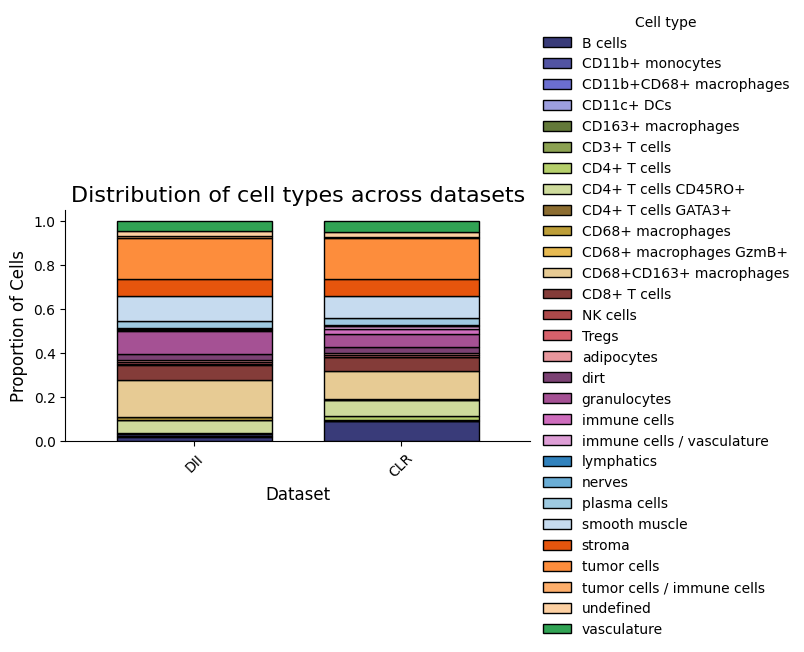
4. Cell Type Composition

from matplotlib.colors import ListedColormap
import matplotlib.cm as cm

# Combine tab20b + tab20c for 40 unique colors
all_colors = []
for name in ["tab20b", "tab20c"]:
    cmap = cm.get_cmap(name)
    all_colors.extend([cmap(i) for i in range(cmap.N)])

seen = set()
unique_colors = []
for c in all_colors:
    key = tuple(round(v, 4) for v in c)
    if key not in seen:
        seen.add(key)
        unique_colors.append(c)

custom_cmap = ListedColormap(unique_colors, name="tab40")

spm.plot_cell_type_distribution(colormap=custom_cmap)

/var/folders/wl/y90xsxr94l78931lqz6nyvz80000gp/T/ipykernel_18164/676858651.py:7: MatplotlibDeprecationWarning: The get_cmap function was deprecated in Matplotlib 3.7 and will be removed in 3.11. Use ``matplotlib.colormaps[name]`` or ``matplotlib.colormaps.get_cmap()`` or ``pyplot.get_cmap()`` instead.
  cmap = cm.get_cmap(name)
/var/folders/wl/y90xsxr94l78931lqz6nyvz80000gp/T/ipykernel_18164/676858651.py:7: MatplotlibDeprecationWarning: The get_cmap function was deprecated in Matplotlib 3.7 and will be removed in 3.11. Use ``matplotlib.colormaps[name]`` or ``matplotlib.colormaps.get_cmap()`` or ``pyplot.get_cmap()`` instead.
  cmap = cm.get_cmap(name)
/Users/sa3520/BWH/spatial query/python/SpatialQuery/spatial_query_multiple_fov.py:1441: MatplotlibDeprecationWarning: The get_cmap function was deprecated in Matplotlib 3.7 and will be removed in 3.11. Use ``matplotlib.colormaps[name]`` or ``matplotlib.colormaps.get_cmap()`` or ``pyplot.get_cmap()`` instead.
  cmap = cm.get_cmap(colormap)

5. Motif Enrichment by Condition

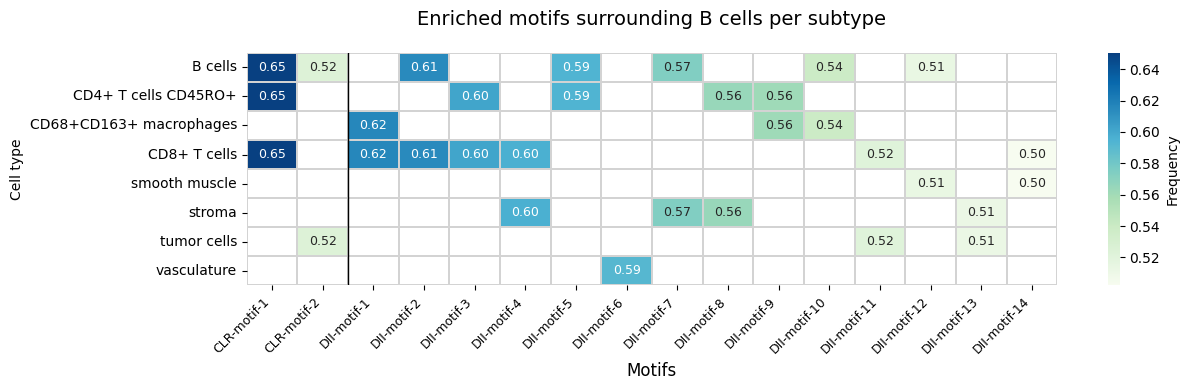
Discover enriched motifs surrounding B cells in each immune subtype separately, then compare the results side by side.

anchor_ct = 'B cells'
max_dist = 5
min_support = 0.5

clr = 'CLR'
dii = 'DII'

enrich_motif_dataset = dict()

for ds in [clr, dii]:
    enrich_motif_dataset[ds] = spm.motif_enrichment_dist(
        ct=anchor_ct,
        dataset=ds,
        max_dist=max_dist,
        min_support=min_support,
        return_cellID=False
    )
    enrich_motif_dataset[ds] = enrich_motif_dataset[ds][enrich_motif_dataset[ds]['if_significant']]
    print(f"Found {len(enrich_motif_dataset[ds])} enriched motifs in {ds}")

enrich_motif_dataset_df = pd.DataFrame()
for ds, df in enrich_motif_dataset.items():
    df['dataset'] = ds
    enrich_motif_dataset_df = pd.concat([enrich_motif_dataset_df, df], axis=0)

Found 2 enriched motifs in CLR
Found 14 enriched motifs in DII

enrich_motif_dataset_df

	center	motifs	n_center_motif	n_center	n_motif	expectation	p-values	adj-pval	if_significant	dataset
0	B cells	[B cells, CD4+ T cells CD45RO+, CD8+ T cells]	6680	10269	27291	2523.399564	0.000000e+00	0.000000e+00	True	CLR
1	B cells	[B cells, tumor cells]	5382	10269	24255	2242.682805	0.000000e+00	0.000000e+00	True	CLR
0	B cells	[B cells, CD8+ T cells]	1704	2774	26742	503.531726	0.000000e+00	0.000000e+00	True	DII
1	B cells	[B cells, CD4+ T cells CD45RO+]	1647	2774	24170	455.102902	0.000000e+00	0.000000e+00	True	DII
2	B cells	[B cells, stroma]	1592	2774	26083	491.123252	0.000000e+00	0.000000e+00	True	DII
3	B cells	[B cells, CD68+CD163+ macrophages]	1495	2774	30610	576.363254	0.000000e+00	0.000000e+00	True	DII
4	B cells	[B cells, smooth muscle]	1425	2774	19963	375.888260	0.000000e+00	0.000000e+00	True	DII
5	B cells	[CD4+ T cells CD45RO+, CD8+ T cells]	1668	2774	58370	1099.063153	1.527325e-107	3.818311e-107	True	DII
6	B cells	[CD8+ T cells, smooth muscle]	1393	2774	47767	899.416646	1.183362e-85	2.535775e-85	True	DII
7	B cells	[CD4+ T cells CD45RO+, stroma]	1566	2774	57711	1086.654679	3.314561e-77	6.214802e-77	True	DII
8	B cells	[CD8+ T cells, stroma]	1655	2774	64677	1217.819215	7.365512e-64	1.227585e-63	True	DII
9	B cells	[vasculature]	1641	2774	66663	1255.214100	3.938264e-50	5.907396e-50	True	DII
10	B cells	[CD8+ T cells, tumor cells]	1447	2774	61444	1156.944259	1.881974e-29	2.566328e-29	True	DII
11	B cells	[CD4+ T cells CD45RO+, CD68+CD163+ macrophages]	1557	2774	70499	1327.443091	5.381246e-19	6.726557e-19	True	DII
12	B cells	[CD68+CD163+ macrophages, CD8+ T cells]	1709	2774	82157	1546.954454	1.412683e-10	1.630019e-10	True	DII
13	B cells	[stroma, tumor cells]	1419	2774	69652	1311.494719	1.712935e-05	1.835287e-05	True	DII

enrich = enrich_motif_dataset_df.copy()
enrich["frequency"] = enrich["n_center_motif"] / enrich["n_center"]

# Sort by dataset, then by frequency within each dataset
enrich = enrich.sort_values(by=["dataset", "frequency"], ascending=[True, False]).reset_index(drop=True)

# Assign motif labels per dataset
enrich["motif_num"] = enrich.groupby("dataset").cumcount() + 1
enrich["motif_group"] = enrich["dataset"] + "_motif_" + enrich["motif_num"].astype(str)

# Build heatmap: cell types × motif groups
enrich_expanded = enrich.explode("motifs")
heatmap_data = enrich_expanded.pivot_table(
    index="motifs", columns="motif_group", values="frequency", aggfunc="first"
)

col_order = enrich["motif_group"].tolist()
heatmap_data = heatmap_data[col_order]
heatmap_data.columns = [col.replace("_", "-") for col in heatmap_data.columns]

# Reorder columns by dataset
clr, dii = "CLR", "DII"
col_order_reordered = []
for ds in [clr, dii]:
    col_order_reordered.extend([c for c in heatmap_data.columns if c.startswith(ds)])
heatmap_data = heatmap_data.loc[:, col_order_reordered]

# Find dataset boundaries for separator lines
boundaries = []
prev_dataset = None
for i, col in enumerate(col_order_reordered):
    current_dataset = col.split("-motif")[0]
    if prev_dataset is not None and current_dataset != prev_dataset:
        boundaries.append(i)
    prev_dataset = current_dataset

# Plot
fig, ax = plt.subplots(figsize=(max(8, len(col_order_reordered) * 0.8), max(4, len(heatmap_data) * 0.45)))
sns.heatmap(
    heatmap_data, cmap="GnBu", linewidths=0.1, linecolor="lightgrey",
    annot=True, fmt=".2f", annot_kws={"fontsize": 9},
    cbar_kws={"label": "Frequency"}, ax=ax,
)
for b in boundaries:
    ax.axvline(x=b, color="black", linewidth=1)

plt.title(f"Enriched motifs surrounding {anchor_ct} per subtype", fontsize=14, pad=20)
plt.ylabel("Cell type")
plt.xlabel("Motifs", fontsize=12)
plt.xticks(rotation=45, ha="right", fontsize=9)
plt.yticks(rotation=0, fontsize=10)
plt.tight_layout()
plt.show()

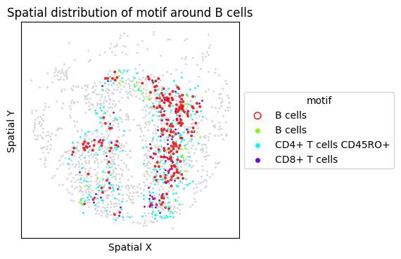
6. Targeted Motif Analysis: Tertiary Lymphoid Structures (TLS)

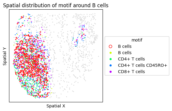
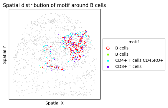
TLS are organized immune aggregates associated with anti-tumor immunity. We test a TLS-associated motif (B cells + T cell subsets) and visualize the FOVs with the highest motif frequency.

motif_tls = ["B cells", "CD4+ T cells", "CD4+ T cells CD45RO+", "CD8+ T cells"]

motif_bcell, id_motif, id_center = spm.motif_enrichment_dist(
    ct=anchor_ct,
    motifs=motif_tls,
    dataset=clr,
    max_dist=max_dist,
    return_cellID=True
)

freq = {
    clr: [],
}
freq_ds_names = {
    clr: [],
}

for sp in spm.spatial_queries:
    sp_ds_name = sp.dataset.split('_')[0]
    if sp_ds_name == clr:
        if anchor_ct not in sp.labels.values:
            continue

        out = sp.motif_enrichment_dist(
            ct=anchor_ct,
            motifs=motif_tls,
            max_dist=max_dist,
            return_cellID=False
        )
        if len(out) == 0:
            continue
        ratio = out['n_center_motif'] / out['n_center']

        if isinstance(ratio, (pd.Series, np.ndarray)):
            ratio = ratio.iloc[0] if hasattr(ratio, "iloc") else ratio.item()

        ratio = float(ratio)

        freq[sp_ds_name].append(ratio)
        freq_ds_names[sp_ds_name].append(sp.dataset)

Found no ['CD4+ T cells'] in ClusterName. Ignoring them.
Found no ['CD4+ T cells'] in ClusterName. Ignoring them.
Found no ['CD4+ T cells'] in ClusterName. Ignoring them.
Found no ['CD4+ T cells'] in ClusterName. Ignoring them.
Found no ['CD4+ T cells'] in ClusterName. Ignoring them.
Found no ['CD4+ T cells'] in ClusterName. Ignoring them.
Found no ['CD4+ T cells'] in ClusterName. Ignoring them.
Found no ['CD4+ T cells'] in ClusterName. Ignoring them.
Found no ['CD4+ T cells'] in ClusterName. Ignoring them.
Found no ['CD4+ T cells'] in ClusterName. Ignoring them.
... (16 lines omitted) ...
Found no ['CD4+ T cells'] in ClusterName. Ignoring them.
Found no ['CD4+ T cells'] in ClusterName. Ignoring them.

def get_top3_names(freq, freq_ds_names, k=3):
    """Return dataset names of the top-k FOVs by motif frequency."""
    result = {}
    for key in freq:
        paired = sorted(zip(freq[key], freq_ds_names[key]), reverse=True)[:k]
        result[key] = [name for _, name in paired]
    return result

top3 = get_top3_names(freq, freq_ds_names)
top3

{'CLR': ['CLR_20', 'CLR_14', 'CLR_28']}

for sp in spm.spatial_queries:
    if sp.dataset in top3[clr]:
        sp.plot_motif_celltype(
            ct=anchor_ct,
            motif=motif_tls,
            max_dist=max_dist,
            figsize=(4, 4),
        )

Found no ['CD4+ T cells'] in ClusterName. Ignoring them.

Found no ['CD4+ T cells'] in ClusterName. Ignoring them.

7. Differential Motif Analysis

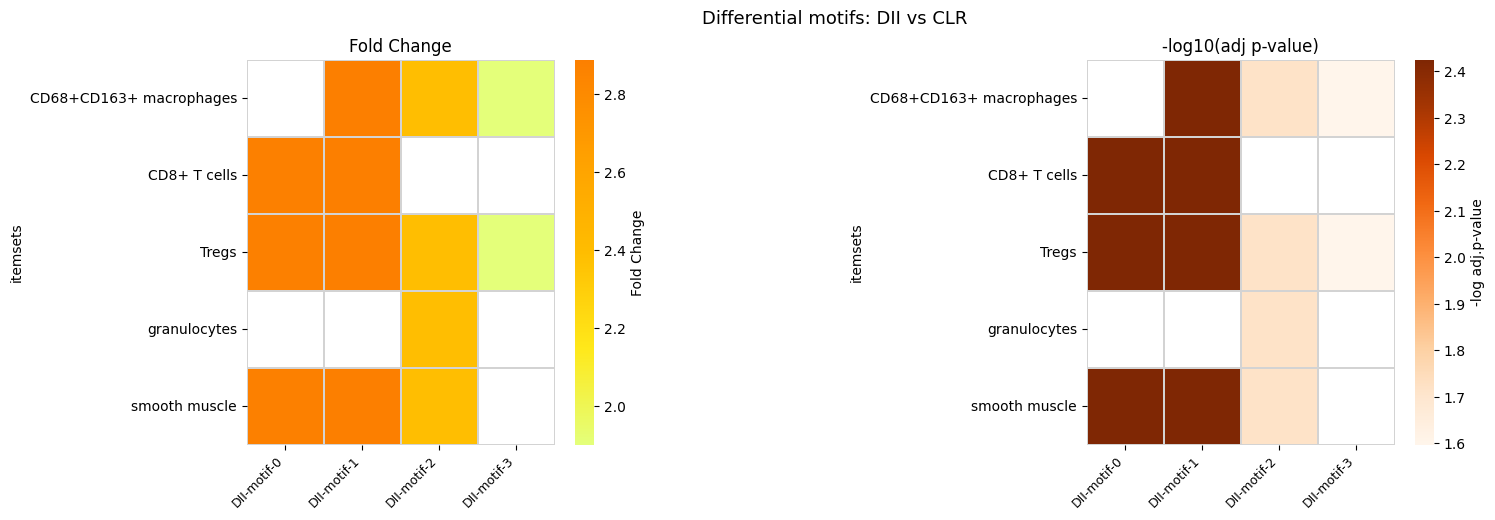
Identify motifs whose frequency differs significantly between CLR and DII subtypes using differential_analysis_dist.

diff_motif_bcell = spm.differential_analysis_dist(
    ct=anchor_ct,
    datasets=[clr, dii],
    max_dist=max_dist,
    min_support=min_support
)

Discovered 501 motifs across the datasets for differential analysis.

diff_motif_bcell[clr]

	itemsets	support_CLR_mean	support_DII_mean	adj-pval

diff_motif_bcell[dii]

	itemsets	support_CLR_mean	support_DII_mean	adj-pval
0	(CD8+ T cells, Tregs, smooth muscle)	0.050989	0.146879	0.003753
1	(CD68+CD163+ macrophages, CD8+ T cells, Tregs,...	0.048059	0.138878	0.003753
2	(CD68+CD163+ macrophages, Tregs, granulocytes,...	0.041341	0.098820	0.019282
3	(CD68+CD163+ macrophages, Tregs)	0.159009	0.302162	0.025271

diff_motif_bcell[clr]['group'] = clr
diff_motif_bcell[dii]['group'] = dii

enrich = diff_motif_bcell[dii]
enrich = pd.concat([enrich, diff_motif_bcell[clr]], axis=0)

enrich['fold_change'] = enrich[f'support_{dii}_mean'] / enrich[f'support_{clr}_mean']

enrich['motif_group'] = enrich['group'] + '_motif_' + enrich.index.astype(str)
col_order = enrich['motif_group'].tolist()

enrich_expanded = enrich.explode('itemsets')

heatmap_fc = enrich_expanded.pivot_table(
    index='itemsets', columns='motif_group', values='fold_change'
)[col_order]

heatmap_pval = enrich_expanded.pivot_table(
    index='itemsets', columns='motif_group', values='adj-pval'
)
heatmap_pval = -np.log10(heatmap_pval)[col_order]

col_labels = [c.replace('_', '-') for c in col_order]
heatmap_fc.columns = col_labels
heatmap_pval.columns = col_labels

fig, (ax1, ax2) = plt.subplots(1, 2, figsize=(16, 5), gridspec_kw={'wspace': 1.1})

sns.heatmap(heatmap_fc, cmap='Wistia', linewidths=0.1, linecolor='lightgrey',
            square=True, cbar_kws={'label': 'Fold Change'}, ax=ax1)
ax1.set_title('Fold Change')
ax1.set_xlabel('')
ax1.set_xticklabels(ax1.get_xticklabels(), rotation=45, ha='right', fontsize=9)

sns.heatmap(heatmap_pval, cmap='Oranges', linewidths=0.1, linecolor='lightgrey',
            square=True, cbar_kws={'label': '-log adj.p-value'}, ax=ax2)
ax2.set_title('-log10(adj p-value)')
ax2.set_xlabel('')
ax2.set_xticklabels(ax2.get_xticklabels(), rotation=45, ha='right', fontsize=9)

fig.suptitle(f'Differential motifs: {dii} vs {clr}', fontsize=13)
plt.tight_layout()
plt.show()

8. Targeted Motif Analysis: Immunosuppressive Niche

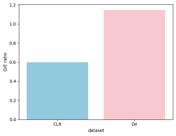
Test a hypothesis-driven immunosuppressive motif (macrophages + Tregs + CD8+ T cells + granulocytes) and compare its enrichment between CLR and DII.

motif_immsup = ["CD68+CD163+ macrophages", "Tregs", "CD8+ T cells", "granulocytes"]

immsup_clr = spm.motif_enrichment_dist(ct=anchor_ct, motifs=motif_immsup, max_dist=max_dist, dataset=clr)
immsup_dii = spm.motif_enrichment_dist(ct=anchor_ct, motifs=motif_immsup, max_dist=max_dist, dataset=dii)

immsup_clr["dataset"] = clr
immsup_dii["dataset"] = dii
immsup_both = pd.concat([immsup_clr, immsup_dii], axis=0)
immsup_both["O/E ratio"] = immsup_both["n_center_motif"] / immsup_both["expectation"]

immsup_both

	center	motifs	n_center_motif	n_center	n_motif	expectation	p-values	if_significant	dataset	O/E ratio
0	B cells	[CD68+CD163+ macrophages, CD8+ T cells, Tregs,...	384	10269	6949	642.523307	1.000000	False	CLR	0.597644
0	B cells	[CD68+CD163+ macrophages, CD8+ T cells, Tregs,...	380	2774	17593	331.262944	0.002119	True	DII	1.147125

sns.barplot(x="dataset", y="O/E ratio", data=immsup_both, palette=["skyblue", "pink"])
plt.show()

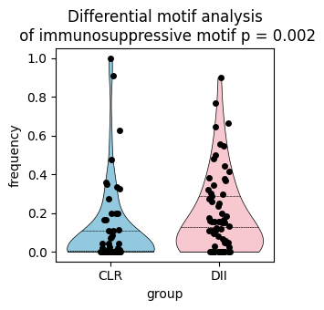
Compute per-FOV motif frequency to test whether the immunosuppressive motif is differentially present between CLR and DII (Mann-Whitney U test).

freq = {clr: [], dii: []}

for sp in spm.spatial_queries:
    sp_ds_name = sp.dataset.split("_")[0]
    if anchor_ct not in sp.labels.values:
        continue

    out = sp.motif_enrichment_dist(
        ct=anchor_ct, motifs=motif_immsup, max_dist=max_dist, return_cellID=False,
    )
    if len(out) == 0:
        continue

    ratio = out["n_center_motif"] / out["n_center"]
    if isinstance(ratio, (pd.Series, np.ndarray)):
        ratio = ratio.iloc[0] if hasattr(ratio, "iloc") else ratio.item()

    freq[sp_ds_name].append(float(ratio))

Found no ['Tregs'] in ClusterName. Ignoring them.
Found no ['Tregs'] in ClusterName. Ignoring them.
Found no ['Tregs'] in ClusterName. Ignoring them.
Found no ['Tregs'] in ClusterName. Ignoring them.
Found no ['Tregs'] in ClusterName. Ignoring them.
Found no ['Tregs'] in ClusterName. Ignoring them.
Found no ['Tregs'] in ClusterName. Ignoring them.

plot_df = pd.DataFrame({
    'group': (
        [clr] * len(freq[clr]) +
        [dii] * len(freq[dii])
    ),
    'frequency': (
        freq[clr] +
        freq[dii]
    )
})

from scipy import stats
group1 = freq[clr]
group2 = freq[dii]
stat, p_value = stats.mannwhitneyu(group1, group2,
                                   alternative='two-sided',
                                   method='auto')

fig, ax = plt.subplots(figsize=(3.2, 3.5))

# Violin
sns.violinplot(
    data=plot_df,
    x="group",
    y="frequency",
    ax=ax,
    cut=0,
    inner="quartile",
    linewidth=0.5,
    edgecolor='black',
    palette=["skyblue", "pink"]
)

# Overlay points
sns.stripplot(
    data=plot_df,
    x="group",
    y="frequency",
    ax=ax,
    color="black",
    size=5,
    jitter=0.1,
)

ax.set_title(f'Differential motif analysis\n of immunosuppressive motif p = {p_value:.3f}')

plt.tight_layout()