Multi-dataset: Gene-Gene Covariation Analysis

This example demonstrates how to identify cross-cell gene-gene covariation across multiple FOVs.

The multi-FOV version pools anchor–neighbor cell pairs across all FOVs within a condition, increasing statistical power for detecting spatially-specific gene correlations.

Dataset: CZI Kidney — normal vs autosomal dominant tubulointerstitial kidney disease (ADTKD) (spatial transcriptomics), availabel at https://cellxgene.cziscience.com/collections/8e880741-bf9a-4c8e-9227-934204631d2a

Key API:

• spatial_query_multi.compute_gene_gene_correlation — pools all non-anchor motif cell types together

• spatial_query_multi.compute_gene_gene_correlation_by_type — tests each non-anchor cell type separately

Tip: For whole-transcriptomic data like this kidney dataset, we’d suggest pre-selecting highly variable genes via the genes parameter to improve speed and reduce multiple-testing burden.

Setup

import warnings
warnings.filterwarnings("ignore")

import os
import anndata as ad
import scanpy as sc
import numpy as np
import matplotlib.pyplot as plt

from SpatialQuery import spatial_query_multi

Load Data & Initialize

DATA_DIR = "../data/CZI_kidney"

data_files = os.listdir(DATA_DIR)
adatas = [ad.read_h5ad(os.path.join(DATA_DIR, f)) for f in data_files]

print(f"Loaded {len(adatas)} FOVs")
adatas[0]

Loaded 84 FOVs

AnnData object with n_obs × n_vars = 12906 × 17811
    obs: 'assay_ontology_term_id', 'self_reported_ethnicity_ontology_term_id', 'is_primary_data', 'organism_ontology_term_id', 'sample', 'tissue_ontology_term_id', 'disease_state', 'sex_ontology_term_id', 'genotype', 'development_stage_ontology_term_id', 'author_cell_type', 'cell_type_ontology_term_id', 'disease_ontology_term_id', 'donor_id', 'suspension_type', 'tissue_type', 'cell_type', 'assay', 'disease', 'organism', 'sex', 'tissue', 'self_reported_ethnicity', 'development_stage', 'observation_joinid'
    var: 'feature_is_filtered', 'feature_name', 'feature_reference', 'feature_biotype', 'feature_length'
    uns: 'citation', 'schema_reference', 'schema_version', 'title'
    obsm: 'X_spatial'

# Create condition labels and filter out mitochondrial / unannotated genes
for i, adata in enumerate(adatas):
    adata.obs['disease_state_genotype'] = (
        adata.obs['disease_state'].astype(str) + '_' + adata.obs['genotype'].astype(str)
    )
    adata.var_names = adata.var['feature_name'].tolist()
    adata = adata[:, ~adata.var_names.str.startswith('mt-')]
    adata = adata[:, ~adata.var_names.str.endswith('Rik')]
    adata = adata[:, ~adata.var_names.str.startswith('Gm')]
    adatas[i] = adata

# Map verbose condition names to short labels
dataset_mapping = {
    'early diabetic kidney disease_BTBR-ob/ob': 'DKD_BTBR-ob/ob',
    'autosomal dominant tubulointersital kidney disease (ADTKD)_UMOD-KI/KI': 'ADTKD_UMOD-KI/KI',
    'control_BTBR-wt/wt': 'control_BTBR-WT/WT',
    'control_UMOD-WT/WT': 'control_UMOD-WT/WT',
}

dataset_name_col = 'disease_state_genotype'
datasets = [adata.obs[dataset_name_col].unique()[0] for adata in adatas]
dataset_names = [dataset_mapping[d] for d in datasets]

spatial_key = "X_spatial"
label_key = "cell_type"
feature_name = 'feature_name'

spm = spatial_query_multi(
    adatas=adatas,
    datasets=dataset_names,
    spatial_key=spatial_key,
    label_key=label_key,
    feature_name=feature_name,
    build_gene_index=False,
    if_lognorm=True,
    if_normalize_spatial_coord=True
)

Replacing _ with hyphen in DKD_BTBR-ob/ob.
Replacing _ with hyphen in DKD_BTBR-ob/ob.
Replacing _ with hyphen in control_BTBR-WT/WT.
Replacing _ with hyphen in control_UMOD-WT/WT.
Replacing _ with hyphen in ADTKD_UMOD-KI/KI.
Replacing _ with hyphen in ADTKD_UMOD-KI/KI.
Replacing _ with hyphen in ADTKD_UMOD-KI/KI.
Replacing _ with hyphen in control_BTBR-WT/WT.
Replacing _ with hyphen in control_BTBR-WT/WT.
Replacing _ with hyphen in DKD_BTBR-ob/ob.
...(492 lines omitted)...
build_gene_index is False. Using adata.X for gene expression analysis.
Log normalizing the expression data... If data is already log normalized, please set if_lognorm to False.

Select Highly Variable Genes

For whole-transcriptomic data, pre-selecting highly variable genes (HVGs) speeds up computation and focuses the analysis on the most informative features.

valid_ds_names = list(set(s.dataset.split('_')[0] for s in spm.spatial_queries))
valid_ds_names

['DKD-BTBR-ob/ob',
 'ADTKD-UMOD-KI/KI',
 'control-BTBR-WT/WT',
 'control-UMOD-WT/WT']

# Select top 3000 HVGs per condition and take the union
tt1 = np.array([f.replace('_','-') for f in dataset_names])
selected_genes = {}
tt2 = []
for adata in adatas:
    adata.var_names = adata.var[feature_name]
    tt2.append(adata)

for ds in valid_ds_names:
    mask = np.where(tt1 == ds)[0]
    adata_sub = ad.concat([tt2[i].copy() for i in mask], join='inner')
    print(f"{ds}: {adata_sub.shape}")
    sc.pp.normalize_total(adata_sub)
    sc.pp.log1p(adata_sub)
    sc.pp.highly_variable_genes(adata_sub, n_top_genes=3000)
    selected_genes[ds] = adata_sub.var[adata_sub.var['highly_variable']].index.tolist()

DKD-BTBR-ob/ob: (613317, 13586)
ADTKD-UMOD-KI/KI: (501021, 14390)
control-BTBR-WT/WT: (550106, 13751)
control-UMOD-WT/WT: (336157, 14271)

Define Anchor and Motif

We use macrophage as the anchor cell type. The motif includes fibroblast and thick ascending limb epithelial cell.

anchor_ct = "macrophage"
motif = ['kidney interstitial fibroblast', 'kidney loop of Henle thick ascending limb epithelial cell']
max_dist = 5
ds_control = 'control-UMOD-WT/WT'
ds_case = 'ADTKD-UMOD-KI/KI'

Method 1: Pooled Covariation (compute_gene_gene_correlation)

compute_gene_gene_correlation pools all non-anchor cell types in the motif into a single neighbor group before computing correlations across FOVs. It performs two tests:

1. Test 1 (spatial specificity): correlation in motif+ anchor–neighbor pairs vs randomly paired cells

2. Test 2 (motif specificity): correlation in motif+ pairs vs motif− anchor–neighbor pairs

Key parameters:

Parameter	Description
ct	Anchor cell type
motif	List of neighbor cell types forming the motif
dataset	Condition name(s) to restrict the analysis to
max_dist	Neighborhood radius (use either max_dist or k)
k	Number of nearest neighbors (use either max_dist or k)
genes	List of genes to analyze. If None, uses all genes
min_nonzero	Minimum non-zero expression values required to include a gene
alpha	FDR significance threshold (default: 0.05)

Key output columns:

Column	Description
gene_center	Gene expressed in the anchor cell
gene_motif	Gene expressed in the neighbor cell
corr_neighbor	Correlation between motif+ anchor–neighbor pairs
corr_non_neighbor	Correlation between randomly paired cells (Test 1 baseline)
corr_center_no_motif	Correlation for motif− anchors (Test 2 baseline)
combined_score	Combined effect size from both tests
if_significant	Whether the pair passes both FDR-corrected tests

covarying_pooled = spm.compute_gene_gene_correlation(
    ct=anchor_ct,
    motif=motif,
    dataset=ds_case,
    max_dist=max_dist,
    genes=selected_genes[ds_case],
    alpha=0.05,
)

covarying_pooled_sig = covarying_pooled[covarying_pooled["if_significant"]].copy()
print(f"Total gene pairs tested: {len(covarying_pooled)}")
print(f"Significant covarying pairs (pooled): {len(covarying_pooled_sig)}")
covarying_pooled_sig.head(10)

Computing covarying genes using expression data ...
Gene coverage: 14390 genes in all FOVs, 18795 genes total (union)
  -> 4405 genes present in subset of FOVs (will use available data)
Analyzing 3000 genes across 24 FOVs

================================================================================
Step 1: Computing and accumulating statistics across FOVs
================================================================================

--- Processing FOV 1/24: ADTKD-UMOD-KI/KI_0 ---
...(177 lines omitted)...
Total gene pairs tested: 9000000
Significant covarying pairs (pooled): 296

	gene_center	gene_motif	corr_neighbor	corr_non_neighbor	p_value_test1	delta_corr_test1	corr_center_no_motif	p_value_test2	delta_corr_test2	combined_score	adj-pval-test1	adj-pval-test2	if_significant
0	Wif1	Wif1	0.312311	-0.011133	0.0	0.323444	-0.000243	0.0	0.312554	94.746418	0.0	0.0	True
1	Armc12	Wif1	0.300108	-0.010945	0.0	0.311053	-0.000126	0.0	0.300234	91.043878	0.0	0.0	True
2	Grid1	Grin3a	0.259830	0.000530	0.0	0.259300	-0.000535	0.0	0.260365	78.013763	0.0	0.0	True
3	Hpdl	Dnah3	0.236931	-0.001030	0.0	0.237962	0.000073	0.0	0.236859	71.156931	0.0	0.0	True
4	Grid1	Myom2	0.221014	-0.000439	0.0	0.221453	0.000255	0.0	0.220759	66.290110	0.0	0.0	True
5	Cercam	Rergl	0.212219	-0.000659	0.0	0.212879	0.004272	0.0	0.207947	62.828013	0.0	0.0	True
6	Kap	Kap	0.368871	-0.012893	0.0	0.381763	0.251811	0.0	0.117059	58.941187	0.0	0.0	True
7	Cyp2d12	Hmx2	0.192851	-0.000510	0.0	0.193361	0.001287	0.0	0.191563	57.630835	0.0	0.0	True
8	Ptprr	Tmc7	0.191837	-0.000012	0.0	0.191850	0.003037	0.0	0.188800	56.914508	0.0	0.0	True
9	Lypd1	Notumos	0.180410	-0.000194	0.0	0.180604	-0.000311	0.0	0.180721	54.205766	0.0	0.0	True

Top Frequent Genes in Covarying Pairs (Pooled)

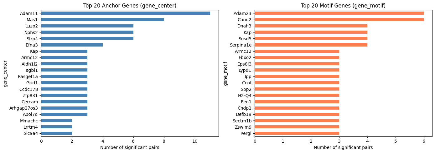
Visualize the top 20 most frequently appearing genes on the anchor side (gene_center) and the motif side (gene_motif) among significant covarying pairs.

top_n = 20

fig, axes = plt.subplots(1, 2, figsize=(14, 5))

covarying_pooled_sig["gene_center"].value_counts().head(top_n).plot.barh(
    ax=axes[0], color="steelblue")
axes[0].set_title(f"Top {top_n} Anchor Genes (gene_center)")
axes[0].set_xlabel("Number of significant pairs")
axes[0].invert_yaxis()

covarying_pooled_sig["gene_motif"].value_counts().head(top_n).plot.barh(
    ax=axes[1], color="coral")
axes[1].set_title(f"Top {top_n} Motif Genes (gene_motif)")
axes[1].set_xlabel("Number of significant pairs")
axes[1].invert_yaxis()

plt.tight_layout()
plt.show()

Method 2: Per-cell-type Covariation (compute_gene_gene_correlation_by_type)

compute_gene_gene_correlation_by_type tests each non-anchor cell type separately, so the output includes a cell_type column.

Key parameters:

Parameter	Description
ct	Anchor cell type
motif	List of neighbor cell types forming the motif
dataset	Condition name(s) to restrict the analysis to. If None, uses all datasets
genes	List of genes to analyze. If None, uses intersection of genes across FOVs
max_dist	Neighborhood radius (use either max_dist or k)
k	Number of nearest neighbors (use either max_dist or k)
min_size	Minimum neighborhood size for each anchor cell
min_nonzero	Minimum non-zero expression values required to include a gene
alpha	FDR significance threshold (default: 0.05)

Key output columns:

Column	Description
cell_type	The neighbor cell type in the pair
gene_center	Gene expressed in the anchor cell
gene_motif	Gene expressed in the neighbor cell
corr_neighbor	Correlation between motif+ anchor–neighbor pairs
corr_non_neighbor	Correlation between randomly paired cells (Test 1 baseline)
corr_center_no_motif	Correlation for motif− anchors (Test 2 baseline)
combined_score	Combined effect size from both tests
if_significant	Whether the pair passes both FDR-corrected tests

covarying = spm.compute_gene_gene_correlation_by_type(
    ct=anchor_ct,
    motif=motif,
    dataset=ds_case,
    max_dist=max_dist,
    genes=selected_genes[ds_case],
    alpha=0.05,
)

covarying_sig = covarying[covarying["if_significant"]].copy()
print(f"Total gene pairs tested: {len(covarying)}")
print(f"Significant covarying pairs: {len(covarying_sig)}")

Computing covarying genes using expression data ...
Analyzing 2 non-center cell types in motif: ['kidney interstitial fibroblast', 'kidney loop of Henle thick ascending limb epithelial cell']
================================================================================
Selected 24 FOVs for analysis
Gene coverage: 14390 genes in all FOVs, 18795 genes total (union)
  -> 4405 genes present in subset of FOVs (will use available data)
Analyzing 3000 genes across 24 FOVs

================================================================================
Step 1: Computing Correlation-3 (Center without motif vs Neighbors)
...(137 lines omitted)...
Total gene pairs tested: 15536862
Significant covarying pairs: 3501

Top Frequent Genes in Covarying Pairs (Per Cell Type)

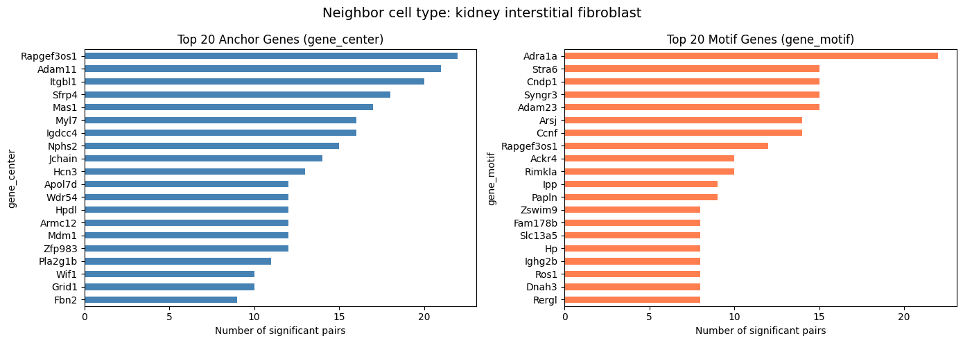
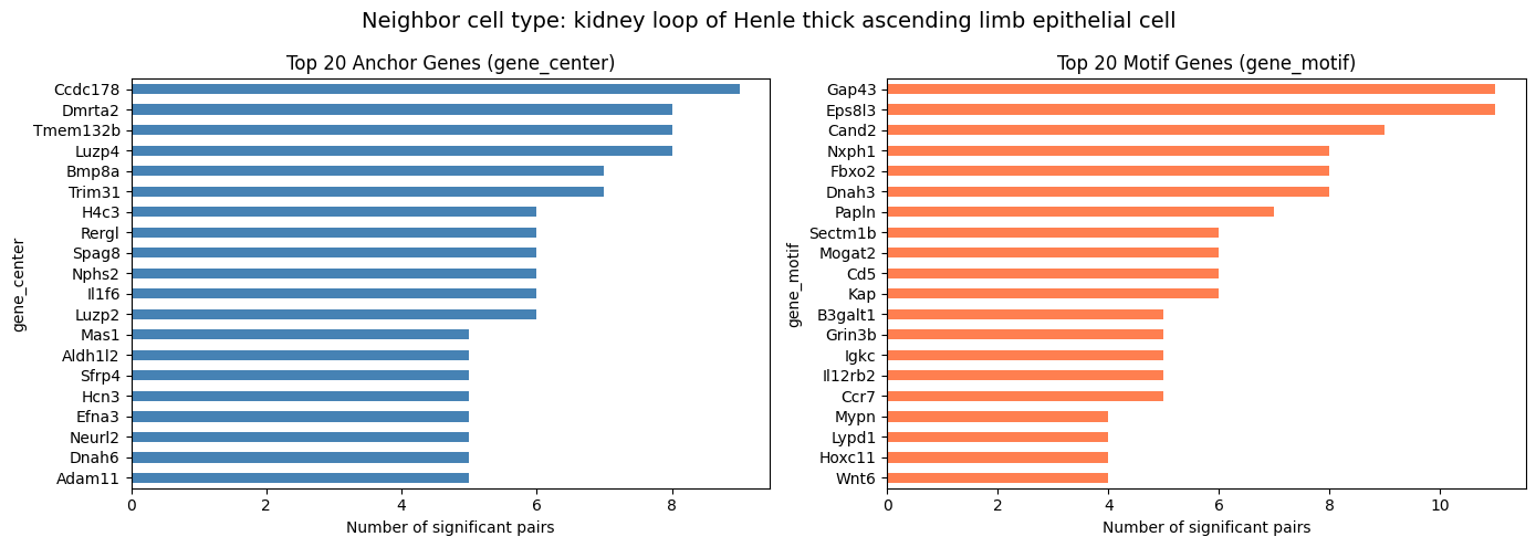
For compute_gene_gene_correlation_by_type, visualize the top 20 genes separately for each neighbor cell type.

top_n = 20
cell_types = covarying_sig["cell_type"].unique()

for ct in cell_types:
    ct_df = covarying_sig[covarying_sig["cell_type"] == ct]
    if len(ct_df) == 0:
        continue

    fig, axes = plt.subplots(1, 2, figsize=(14, 5))
    fig.suptitle(f"Neighbor cell type: {ct}", fontsize=14)

    ct_df["gene_center"].value_counts().head(top_n).plot.barh(
        ax=axes[0], color="steelblue")
    axes[0].set_title(f"Top {top_n} Anchor Genes (gene_center)")
    axes[0].set_xlabel("Number of significant pairs")
    axes[0].invert_yaxis()

    ct_df["gene_motif"].value_counts().head(top_n).plot.barh(
        ax=axes[1], color="coral")
    axes[1].set_title(f"Top {top_n} Motif Genes (gene_motif)")
    axes[1].set_xlabel("Number of significant pairs")
    axes[1].invert_yaxis()

    plt.tight_layout()
    plt.show()

Summary by Neighbor Cell Type

covarying_sig["cell_type"].value_counts()

cell_type
kidney interstitial fibroblast                               2525
kidney loop of Henle thick ascending limb epithelial cell     976
Name: count, dtype: int64

Inspect Top Covarying Gene Pairs

Sort by combined score (absolute value) to see the strongest associations.

covarying_sig.sort_values("abs_combined_score", ascending=False).head(10)

	cell_type	gene_center	gene_motif	corr_neighbor	corr_non_neighbor	p_value_test1	delta_corr_test1	corr_center_no_motif	p_value_test2	delta_corr_test2	combined_score	q_value_test1	q_value_test2	reject_test1_fdr	reject_test2_fdr	abs_combined_score	if_significant
0	kidney interstitial fibroblast	Wif1	Lmo3	0.815627	-0.020971	0.0	0.836598	-0.000371	0.0	0.815997	246.653183	0.0	0.0	True	True	246.653183	True
1	kidney interstitial fibroblast	Wif1	Wif1	0.786223	-0.035668	0.0	0.821892	-0.000243	0.0	0.786467	239.128233	0.0	0.0	True	True	239.128233	True
2	kidney interstitial fibroblast	Armc12	Lmo3	0.748789	-0.020264	0.0	0.769053	-0.000078	0.0	0.748867	226.476755	0.0	0.0	True	True	226.476755	True
3	kidney interstitial fibroblast	Rapgef3os1	Slamf1	0.742925	-0.017139	0.0	0.760064	-0.000098	0.0	0.743023	224.440595	0.0	0.0	True	True	224.440595	True
4	kidney interstitial fibroblast	Armc12	Wif1	0.721795	-0.034466	0.0	0.756261	-0.000126	0.0	0.721921	219.666989	0.0	0.0	True	True	219.666989	True
5	kidney interstitial fibroblast	Luzp2	Serpina1e	0.699316	-0.024935	0.0	0.724251	0.005572	0.0	0.693744	210.868927	0.0	0.0	True	True	210.868927	True
6	kidney interstitial fibroblast	Rapgef3os1	Cerox1	0.671484	-0.019855	0.0	0.691338	-0.000087	0.0	0.671571	203.250420	0.0	0.0	True	True	203.250420	True
7	kidney interstitial fibroblast	Fam178b	Ppp1r3d	0.601521	-0.000445	0.0	0.601967	-0.000137	0.0	0.601659	180.525313	0.0	0.0	True	True	180.525313	True
8	kidney interstitial fibroblast	Gap43	Best3	0.528982	-0.016956	0.0	0.545937	-0.000250	0.0	0.529231	160.272942	0.0	0.0	True	True	160.272942	True
9	kidney interstitial fibroblast	Cercam	Rergl	0.493953	-0.001935	0.0	0.495888	0.004272	0.0	0.489681	147.462958	0.0	0.0	True	True	147.462958	True

Visualize Covarying Gene Modules

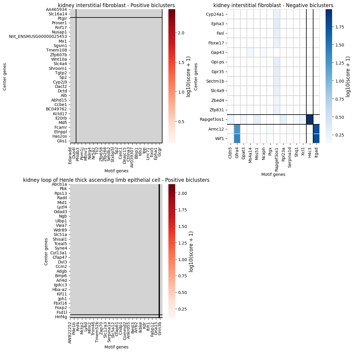
Note: plot_gene_pair_heatmap is available on the single-dataset spatial_query class. For multi-dataset results, you can use the standalone plotting function from SpatialQuery.plotting or apply clustering directly to the result DataFrame.

from SpatialQuery.plotting import plot_gene_pair_heatmap

if len(covarying_sig) > 0:
    modules = plot_gene_pair_heatmap(
        gene_pair_df=covarying_sig,
        figsize=(12, 6),
    )
else:
    print("No significant covarying gene pairs found.")

kidney loop of Henle thick ascending limb epithelial cell: Skipping neg with 4 rows and 1 columns.

modules

	gene_center	gene_motif	combined_score	cluster_type	cluster_row	cluster_col	cell_type
0	AA465934	Adamts7	25.321869	positive	0	1	kidney interstitial fibroblast
1	AA465934	Il12rb2	26.951418	positive	0	1	kidney interstitial fibroblast
2	AA465934	Tmem143	1.009324	positive	0	1	kidney interstitial fibroblast
3	AA914427	Dgki	0.660621	positive	1	1	kidney interstitial fibroblast
4	AA914427	Iqcm	0.763277	positive	1	1	kidney interstitial fibroblast
...	...	...	...	...	...	...	...
3492	Zfp983	Eps8l3	42.379554	positive	0	2	kidney loop of Henle thick ascending limb epit...
3493	Zfp991	Nuggc	0.338234	positive	0	0	kidney loop of Henle thick ascending limb epit...
3494	Zfp992	B3galt1	0.399425	positive	0	0	kidney loop of Henle thick ascending limb epit...
3495	Zfp992	Sectm1b	0.568542	positive	0	0	kidney loop of Henle thick ascending limb epit...
3496	Zkscan5	Mypn	0.492021	positive	0	0	kidney loop of Henle thick ascending limb epit...

3497 rows × 7 columns