Multi-dataset: Differential Motif Analysis

This example demonstrates how to identify motifs that are differentially enriched between two experimental conditions using differential_analysis_dist.

While motif enrichment (previous example) discovers motifs within each condition independently, differential motif analysis directly compares motif frequencies between conditions using a Mann-Whitney U test across FOVs, with FDR correction for multiple testing.

Dataset: CODEX spatial proteomics — CLR vs DII immune subtypes Key API: spatial_query_multi.differential_analysis_dist and spatial_query_multi.differential_analysis_knn

Setup

[1]:

import warnings
warnings.filterwarnings("ignore")

import anndata as ad
import numpy as np
import pandas as pd
import matplotlib.pyplot as plt
import seaborn as sns

from SpatialQuery import spatial_query_multi

Load Data & Initialize

[3]:

DATA_DIR = "../data/codex_cancer"

adata = ad.read_h5ad(f"{DATA_DIR}/codex_data.h5ad")

adata

[3]:

AnnData object with n_obs × n_vars = 258385 × 56
    obs: 'CellID', 'ClusterID', 'EventID', 'File Name', 'Region', 'TMA_AB', 'TMA_12', 'Index in File', 'groups', 'patients', 'spots', 'cell_id', 'size:size', 'HOECHST1_Cyc_1_ch_1', 'DRAQ5_Cyc_23_ch_4', 'Profile_Homogeneity:Fiter1', 'ClusterSize', 'ClusterName', 'neighborhood10', 'CD4+ICOS+', 'CD4+Ki67+', 'CD4+PD-1+', 'CD68+CD163+ICOS+', 'CD68+CD163+Ki67+', 'CD68+CD163+PD-1+', 'CD68+ICOS+', 'CD68+Ki67+', 'CD68+PD-1+', 'CD8+ICOS+', 'CD8+Ki67+', 'CD8+PD-1+', 'Treg-ICOS+', 'Treg-Ki67+', 'Treg-PD-1+', 'neighborhood number final', 'neighborhood name'
    var: 'marker_name', 'full_name', 'cell_type_annotation', 'cycle', 'channel'
    uns: 'data_source', 'groups_mapping', 'n_markers', 'technology'
    obsm: 'X_spatial_global', 'X_spatial_tile'

[4]:

adata.X.max()

[4]:

np.float32(54776.695)

Inspect adata.obsm for spatial coordinates, adata.obs for cell type labels and FOV identifiers, and adata.var for feature names. Then set the corresponding column names below.

[5]:

# Assign immune subtype labels
adata.obs["state"] = "CLR"
adata.obs["state"][adata.obs["groups"] == 2] = "DII"

# Feature-wise z-score normalization for protein expression
adata.X = (adata.X - adata.X.mean(axis=0)) / adata.X.std(axis=0)

[6]:

spatial_key = "X_spatial_tile"
label_key = "ClusterName"
feature_name = "marker_name"
fov_key = "File Name"

[7]:

# Split data by FOV and immune subtype
clr_data = adata[adata.obs["state"] == "CLR"]
dii_data = adata[adata.obs["state"] == "DII"]

clr_datas = [clr_data[clr_data.obs[fov_key] == f] for f in clr_data.obs[fov_key].unique()]
dii_datas = [dii_data[dii_data.obs[fov_key] == f] for f in dii_data.obs[fov_key].unique()]

ds_names = ["CLR"] * len(clr_datas) + ["DII"] * len(dii_datas)
adata_fovs = clr_datas + dii_datas

print(f"CLR FOVs: {len(clr_datas)}, DII FOVs: {len(dii_datas)}")

CLR FOVs: 68, DII FOVs: 72

[8]:

spm = spatial_query_multi(
    adatas=adata_fovs,
    datasets=ds_names,
    spatial_key=spatial_key,
    label_key=label_key,
    feature_name=feature_name,
    build_gene_index=False,
    if_lognorm=False,  # data is already z-score normalized
    if_normalize_spatial_coord=True,
)


Auto-normalizing spatial coordinates: mean nearest neighbor distance = 1.0
Scale factor: 0.0448
build_gene_index is False. Using adata.X for gene expression analysis.

Auto-normalizing spatial coordinates: mean nearest neighbor distance = 1.0
Scale factor: 0.0311
build_gene_index is False. Using adata.X for gene expression analysis.

Auto-normalizing spatial coordinates: mean nearest neighbor distance = 1.0
... (548 lines omitted) ...
Scale factor: 0.0421
build_gene_index is False. Using adata.X for gene expression analysis.

Run Differential Motif Analysis

differential_analysis_dist compares motif frequencies between two conditions across FOVs. It first discovers all motifs present in either condition, then tests whether the per-FOV support (frequency) of each motif differs significantly.

Key parameters:

Parameter	Description
`ct`	Anchor cell type
`datasets`	List of exactly two condition names to compare
`max_dist`	Neighborhood radius
`min_support`	Minimum support threshold for motif mining

Return value: A dictionary with one key per condition. Each value is a DataFrame of motifs that are significantly more frequent in that condition.

Output columns:

Column	Description
`itemsets`	The motif (frozenset of cell types)
`support_<cond1>_mean`	Mean frequency across FOVs in condition 1
`support_<cond2>_mean`	Mean frequency across FOVs in condition 2
`adj-pval`	FDR-adjusted p-value (Mann-Whitney U)

[9]:

anchor_ct = "B cells"
max_dist = 5
min_support = 0.5
clr = "CLR"
dii = "DII"

diff_motif = spm.differential_analysis_dist(
    ct=anchor_ct,
    datasets=[clr, dii],
    max_dist=max_dist,
    min_support=min_support,
)

Discovered 501 motifs across the datasets for differential analysis.

Inspect Results

Check which motifs are enriched in each condition.

[10]:

print(f"Motifs enriched in {clr}: {len(diff_motif[clr])}")
diff_motif[clr]

Motifs enriched in CLR: 0

[10]:

	itemsets	support_CLR_mean	support_DII_mean	adj-pval

[11]:

print(f"Motifs enriched in {dii}: {len(diff_motif[dii])}")
diff_motif[dii]

Motifs enriched in DII: 4

[11]:

	itemsets	support_CLR_mean	support_DII_mean	adj-pval
0	(CD8+ T cells, Tregs, smooth muscle)	0.050989	0.146879	0.003753
1	(CD68+CD163+ macrophages, CD8+ T cells, Tregs,...	0.048059	0.138878	0.003753
2	(CD68+CD163+ macrophages, Tregs, granulocytes,...	0.041341	0.098820	0.019282
3	(CD68+CD163+ macrophages, Tregs)	0.159009	0.302162	0.025271

Validate Differential Motifs with Enrichment Analysis

A motif being differential (more frequent in one condition) does not guarantee it is enriched (significantly over-represented compared to random expectation) in that condition. To confirm, run motif_enrichment_dist on the differential motifs within the condition where they are more frequent.

[12]:

for ds in [clr, dii]:
    df = diff_motif[ds]
    if len(df) == 0:
        print(f"{ds}: No differential motifs to validate.\n")
        continue

    # Extract motif lists from the differential results
    motif_lists = [list(m) for m in df["itemsets"]]

    enrich_result = spm.motif_enrichment_dist(
        ct=anchor_ct,
        motifs=motif_lists,
        dataset=ds,
        max_dist=max_dist,
        min_support=min_support,
    )

    n_enriched = enrich_result["if_significant"].sum()
    print(f"{ds}: {len(df)} differential motifs → {n_enriched} also enriched")
    display(enrich_result)

CLR: No differential motifs to validate.

DII: 4 differential motifs → 4 also enriched

	center	motifs	n_center_motif	n_center	n_motif	expectation	p-values	adj-pval	if_significant
0	B cells	[CD8+ T cells, Tregs, smooth muscle]	524	2774	14684	276.488664	4.919139e-47	1.967656e-46	True
1	B cells	[CD68+CD163+ macrophages, CD8+ T cells, Tregs,...	390	2774	13610	256.266053	4.003156e-17	8.006311e-17	True
2	B cells	[CD68+CD163+ macrophages, Tregs]	758	2774	33568	632.060167	7.534204e-09	1.004561e-08	True
3	B cells	[CD68+CD163+ macrophages, Tregs, granulocytes,...	269	2774	12513	235.610369	1.094891e-02	1.094891e-02	True

KNN-based Differential Motif Analysis

The KNN variant (differential_analysis_knn) defines neighborhoods by the k nearest neighbors rather than a fixed radius. This can provide complementary results, especially when cell density varies.

[13]:

k = 30

diff_motif_knn = spm.differential_analysis_knn(
    ct=anchor_ct,
    datasets=[clr, dii],
    k=k,
    min_support=min_support,
)

for ds in [clr, dii]:
    print(f"KNN differential motifs in {ds}: {len(diff_motif_knn[ds])}")

KNN differential motifs in CLR: 0
KNN differential motifs in DII: 4

[14]:

diff_motif_knn[clr]

[14]:

	itemsets	support_CLR_mean	support_DII_mean	adj-pval

[15]:

diff_motif_knn[dii]

[15]:

	itemsets	support_CLR_mean	support_DII_mean	adj-pval
0	(CD68+CD163+ macrophages, Tregs, smooth muscle)	0.058319	0.179174	0.023677
1	(CD4+ T cells CD45RO+, CD68+CD163+ macrophages...	0.107069	0.245905	0.023677
2	(CD4+ T cells CD45RO+, CD68+CD163+ macrophages...	0.032668	0.118155	0.023677
3	(CD4+ T cells CD45RO+, CD68+CD163+ macrophages...	0.093074	0.211532	0.030161

Validate KNN Differential Motifs with Enrichment Analysis

Same validation as above, but using motif_enrichment_knn to match the KNN neighborhood definition used in differential analysis.

[16]:

for ds in [clr, dii]:
    df = diff_motif_knn[ds]
    if len(df) == 0:
        print(f"{ds}: No differential motifs to validate.\n")
        continue

    motif_lists = [list(m) for m in df["itemsets"]]

    enrich_result = spm.motif_enrichment_knn(
        ct=anchor_ct,
        motifs=motif_lists,
        dataset=ds,
        k=k,
    )

    n_enriched = enrich_result["if_significant"].sum()
    print(f"{ds}: {len(df)} differential motifs → {n_enriched} also enriched")
    display(enrich_result)

CLR: No differential motifs to validate.

DII: 4 differential motifs → 4 also enriched

	center	motifs	n_center_motif	n_center	n_motif	expectation	p-values	adj-pval	if_significant
0	B cells	[CD4+ T cells CD45RO+, CD68+CD163+ macrophages...	535	2774	24457	460.506896	0.000075	0.000171	True
1	B cells	[CD4+ T cells CD45RO+, CD68+CD163+ macrophages...	256	2774	10846	204.222014	0.000102	0.000171	True
2	B cells	[CD4+ T cells CD45RO+, CD68+CD163+ macrophages...	438	2774	19761	372.084752	0.000128	0.000171	True
3	B cells	[CD68+CD163+ macrophages, Tregs, smooth muscle]	435	2774	20771	391.102292	0.007858	0.007858	True

Built-in Visualization

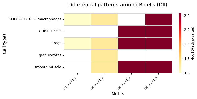
SpatialQuery provides plot_differential_pattern_heatmap for quick visualization of differential motif results.

[18]:

from SpatialQuery.plotting import plot_differential_pattern_heatmap

plot_differential_pattern_heatmap(diff_motif=diff_motif, ct=anchor_ct)

../_images/examples_multi_differential_motif_25_0.png

Custom Visualization

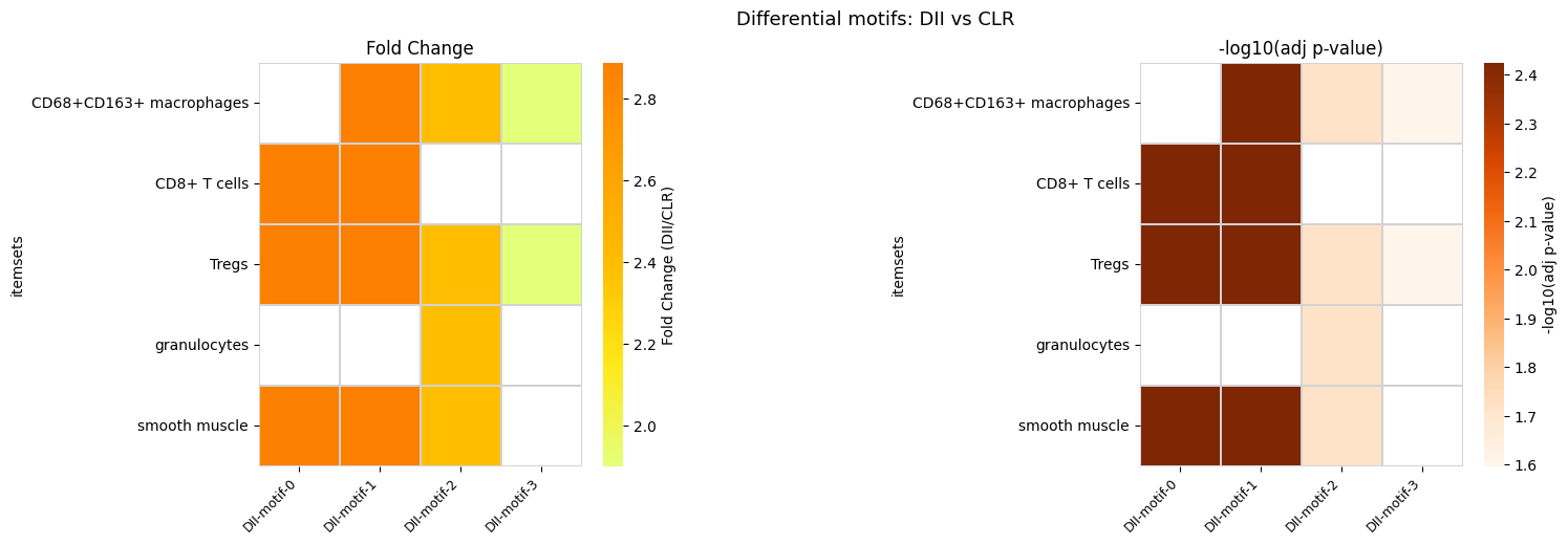
For more control over the layout, you can build custom heatmaps from the result DataFrame. Below we create side-by-side fold change and significance heatmaps.

[19]:

diff_motif[clr] = diff_motif[clr].copy()
diff_motif[dii] = diff_motif[dii].copy()
diff_motif[clr]["group"] = clr
diff_motif[dii]["group"] = dii

enrich = pd.concat([diff_motif[dii], diff_motif[clr]], axis=0)
enrich["fold_change"] = enrich[f"support_{dii}_mean"] / enrich[f"support_{clr}_mean"]
enrich["motif_group"] = enrich["group"] + "_motif_" + enrich.index.astype(str)
col_order = enrich["motif_group"].tolist()

enrich_expanded = enrich.explode("itemsets")

heatmap_fc = enrich_expanded.pivot_table(
    index="itemsets", columns="motif_group", values="fold_change",
)[col_order]

heatmap_pval = enrich_expanded.pivot_table(
    index="itemsets", columns="motif_group", values="adj-pval",
)
heatmap_pval = -np.log10(heatmap_pval)[col_order]

col_labels = [c.replace("_", "-") for c in col_order]
heatmap_fc.columns = col_labels
heatmap_pval.columns = col_labels

fig, (ax1, ax2) = plt.subplots(1, 2, figsize=(16, 5), gridspec_kw={"wspace": 1.1})

sns.heatmap(
    heatmap_fc, cmap="Wistia", linewidths=0.1, linecolor="lightgrey",
    square=True, cbar_kws={"label": "Fold Change (DII/CLR)"}, ax=ax1,
)
ax1.set_title("Fold Change")
ax1.set_xlabel("")
ax1.set_xticklabels(ax1.get_xticklabels(), rotation=45, ha="right", fontsize=9)

sns.heatmap(
    heatmap_pval, cmap="Oranges", linewidths=0.1, linecolor="lightgrey",
    square=True, cbar_kws={"label": "-log10(adj p-value)"}, ax=ax2,
)
ax2.set_title("-log10(adj p-value)")
ax2.set_xlabel("")
ax2.set_xticklabels(ax2.get_xticklabels(), rotation=45, ha="right", fontsize=9)

fig.suptitle(f"Differential motifs: {dii} vs {clr}", fontsize=13)
plt.tight_layout()
plt.show()

../_images/examples_multi_differential_motif_27_0.png

[ ]: