Single-dataset: Motif Enrichment Analysis

This example demonstrates how to discover and visualize spatial motifs — statistically enriched cell-type co-occurrence patterns — in the neighborhood of a given anchor cell type.

Motif enrichment is the foundational analysis in SpatialQuery. It answers the question: “Which cell-type combinations are found near my cell type of interest more often than expected by chance?”

Dataset: seqFISH mouse organogenesis E8.5 embryo (17,806 cells × 351 genes) Key API: spatial_query.motif_enrichment_dist, spatial_query.motif_enrichment_knn

Setup

import warnings
warnings.filterwarnings("ignore")

import anndata as ad
import numpy as np
import pandas as pd
import matplotlib.pyplot as plt

from SpatialQuery import spatial_query

Load Data

DATA_DIR = "../data/mouse_organogenesis"

adata = ad.read_h5ad(f"{DATA_DIR}/embryo1.h5ad")
adata

AnnData object with n_obs × n_vars = 17806 × 351
    obs: 'embryo', 'pos', 'z', 'x_global', 'y_global', 'x_global_affine', 'y_global_affine', 'embryo_pos', 'embryo_pos_z', 'Area', 'UMAP1', 'UMAP2', 'celltype_mapped_refined', 'segmentation_vertices_x_global_affine', 'segmentation_vertices_y_global_affine'
    var: 'gene'
    uns: 'celltype_mapped_refined_colors'
    obsm: 'X_spatial', 'X_umap'

adata.X

array([[0, 0, 0, ..., 0, 1, 0],
       [0, 2, 0, ..., 0, 0, 1],
       [0, 0, 1, ..., 1, 1, 0],
       ...,
       [2, 2, 0, ..., 1, 3, 1],
       [0, 0, 1, ..., 0, 2, 3],
       [0, 0, 0, ..., 0, 1, 0]], shape=(17806, 351))

Inspect adata.obsm for spatial coordinates, adata.obs for cell type labels, and adata.var for gene names. Then set the corresponding column names below. Data is not normalized.

spatial_key = "X_spatial"
label_key = "celltype_mapped_refined"
feature_name = "gene"
dataset_name = "mouse_embryo1"

Initialize SpatialQuery

sp = spatial_query(
    adata=adata,
    dataset=dataset_name,
    spatial_key=spatial_key,
    label_key=label_key,
    feature_name=feature_name,
    build_gene_index=False,
    if_lognorm=True,
    if_normalize_spatial_coord=True,
)

Auto-normalizing spatial coordinates: mean nearest neighbor distance = 1.0
Scale factor: 51.7200
build_gene_index is False. Using adata.X for gene expression analysis.
Log normalizing the expression data... If data is already log normalized, please set if_lognorm to False.

Visualize the Field of View

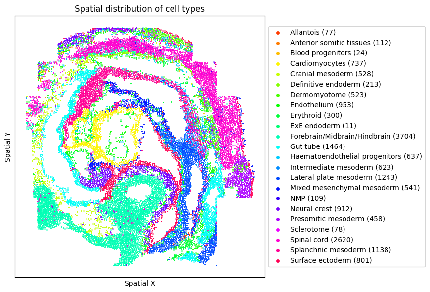
Before running any analysis, it is useful to visualize the spatial distribution of cell types.

sp.plot_fov(min_cells_label=0, figsize=(8, 6))

Unsupervised Motif Discovery

Call motif_enrichment_dist with an anchor cell type to discover all significantly enriched motifs in its neighborhood. The method uses the FP-Growth algorithm to mine frequent cell-type combinations, then tests each for enrichment against a hypergeometric null.

Key parameters:

Parameter	Description
ct	Anchor cell type whose neighborhood is examined
max_dist	Radius of the neighborhood (in normalized spatial units)
min_support	Minimum fraction of anchor cells that must contain the motif

Output columns:

Column	Description
center	The anchor cell type
motifs	List of cell types forming the motif
n_center_motif	Number of anchor cells with this motif in their neighborhood
n_center	Total number of anchor cells
n_motif	Number of cells belonging to the motif cell types
expectation	Expected count under the null (hypergeometric)
p-values	Raw p-value
adj-pval	FDR-corrected p-value (Benjamini-Hochberg). Only present when multiple motifs are tested
if_significant	Whether the motif passes the significance threshold

anchor_ct = "Gut tube"
max_dist = 8

enrich = sp.motif_enrichment_dist(
    ct=anchor_ct,
    max_dist=max_dist,
    min_support=0.2,
)

enrich

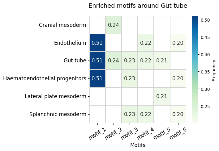
	center	motifs	n_center_motif	n_center	n_motif	expectation	p-values	adj-pval	if_significant
0	Gut tube	[Endothelium, Gut tube, Haematoendothelial pro...	748	1464	2439	200.533303	1.260625e-290	7.563750e-290	True
1	Gut tube	[Cranial mesoderm, Gut tube]	357	1464	1282	105.405369	4.065308e-107	1.219592e-106	True
2	Gut tube	[Endothelium, Gut tube, Splanchnic mesoderm]	320	1464	1188	97.676738	7.788483e-91	1.557697e-90	True
3	Gut tube	[Gut tube, Haematoendothelial progenitors, Spl...	332	1464	1433	117.820510	1.252217e-75	1.878326e-75	True
4	Gut tube	[Gut tube, Lateral plate mesoderm]	312	1464	1595	131.140065	1.212101e-52	1.454521e-52	True
5	Gut tube	[Endothelium, Haematoendothelial progenitors, ...	293	1464	2863	235.394361	1.308209e-05	1.308209e-05	True

Visualize Enriched Motifs

plot_motif_enrichment_heatmap displays which cell types participate in each enriched motif and their frequency of co-occurrence. Each column is a motif, each row is a cell type, and the color intensity indicates the frequency.

sp.plot_motif_enrichment_heatmap(
    enrich_df=enrich,
    figsize=(7, 5),
    title=f"Enriched motifs around {anchor_ct}",
)

KNN-based Motif Enrichment

SpatialQuery provides two neighborhood definitions for motif analysis:

• Distance-based (motif_enrichment_dist): all cells within a fixed radius.

• KNN-based (motif_enrichment_knn): the k nearest neighbors of each anchor cell, optionally capped at max_dist.

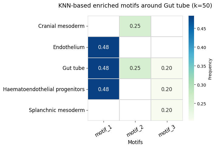
KNN neighborhoods have a fixed size regardless of local cell density, which can be advantageous in datasets with variable cell spacing.

k = 50

enrich_knn = sp.motif_enrichment_knn(
    ct=anchor_ct,
    k=k,
    min_support=0.2,
)

enrich_knn

	center	motifs	n_center_motif	n_center	n_motif	expectation	p-values	adj-pval	if_significant
0	Gut tube	[Endothelium, Gut tube, Haematoendothelial pro...	708	1464	2258	185.651578	8.315571e-278	2.494671e-277	True
1	Gut tube	[Cranial mesoderm, Gut tube]	372	1464	1262	103.760979	9.010722e-121	1.351608e-120	True
2	Gut tube	[Gut tube, Haematoendothelial progenitors, Spl...	298	1464	1243	102.198809	5.899679e-71	5.899679e-71	True

sp.plot_motif_enrichment_heatmap(
    enrich_df=enrich_knn,
    figsize=(7, 5),
    title=f"KNN-based enriched motifs around {anchor_ct} (k={k})",
)

Targeted Motif Enrichment

If you have a specific motif hypothesis (e.g., from literature or prior analysis), you can test it directly by passing the motifs parameter. This skips the FP-Growth mining step and only tests the specified combination.

motif = ["Splanchnic mesoderm", "Endothelium"]

targeted = sp.motif_enrichment_dist(
    ct=anchor_ct,
    motifs=motif,
    max_dist=max_dist,
)

targeted

	center	motifs	n_center_motif	n_center	n_motif	expectation	p-values	if_significant
0	Gut tube	[Endothelium, Splanchnic mesoderm]	322	1464	3117	256.278109	0.000002	True

Or targeted motif enrichment with KNN neighborhoods:

targeted_knn = sp.motif_enrichment_knn(
    ct=anchor_ct,
    motifs=motif,
    k=k,
)

targeted_knn

	center	motifs	n_center_motif	n_center	n_motif	expectation	p-values	if_significant
0	Gut tube	[Endothelium, Splanchnic mesoderm]	289	1464	2845	233.914411	0.000027	True

Spatial Visualization of Motif

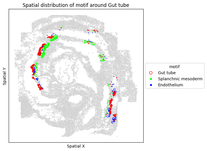
plot_motif_celltype highlights the anchor cells and their motif-associated neighbors on the spatial map. This helps verify that the motif corresponds to biologically meaningful spatial organization.

sp.plot_motif_celltype(
    ct=anchor_ct,
    motif=motif,
    max_dist=max_dist,
    figsize=(6, 6),
)

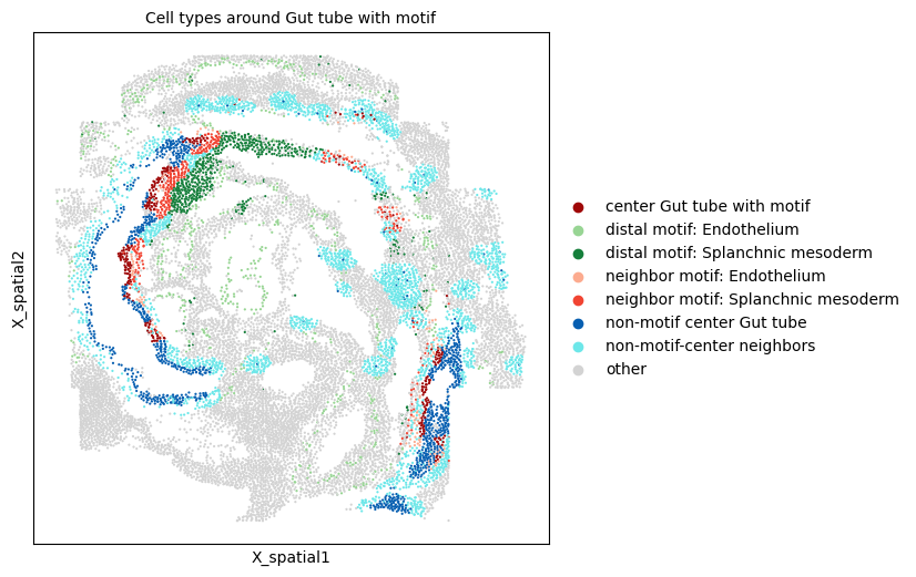
Motif-positive vs Motif-negative Anchor Cells

plot_all_center_motif separates anchor cells into motif-positive (those with the motif in their neighborhood) and motif-negative groups, providing a spatial overview of motif prevalence.

Note: This function requires cell IDs from get_anchor_motif_cell_ids, which internally identifies motif+/motif− groups.

ids = sp.get_anchor_motif_cell_ids(
    ct=anchor_ct,
    motif=motif,
    max_dist=max_dist
)

sp.plot_all_center_motif(
    ct=anchor_ct,
    ids=ids,
)