Single-dataset: Differential Expression Analysis

This example demonstrates how to identify differentially expressed genes between motif-positive and motif-negative anchor cells within a single spatial dataset.

After identifying an enriched motif, SpatialQuery can split anchor cells into two groups: those surrounded by the motif (motif+) and those not (motif−). Comparing gene expression between these groups reveals genes whose expression is associated with specific spatial contexts.

Dataset: seqFISH mouse organogenesis E8.5 embryo (17,806 cells × 351 genes) Key API: spatial_query.de_genes

Setup

import warnings
warnings.filterwarnings("ignore")

import anndata as ad
import numpy as np
import pandas as pd

from SpatialQuery import spatial_query

Load Data & Initialize

DATA_DIR = "../data/mouse_organogenesis"

adata = ad.read_h5ad(f"{DATA_DIR}/embryo1.h5ad")
adata

AnnData object with n_obs × n_vars = 17806 × 351
    obs: 'embryo', 'pos', 'z', 'x_global', 'y_global', 'x_global_affine', 'y_global_affine', 'embryo_pos', 'embryo_pos_z', 'Area', 'UMAP1', 'UMAP2', 'celltype_mapped_refined', 'segmentation_vertices_x_global_affine', 'segmentation_vertices_y_global_affine'
    var: 'gene'
    uns: 'celltype_mapped_refined_colors'
    obsm: 'X_spatial', 'X_umap'

Inspect adata.obsm for spatial coordinates, adata.obs for cell type labels, and adata.var for gene names. Then set the corresponding column names below.

spatial_key = "X_spatial"
label_key = "celltype_mapped_refined"
feature_name = "gene"
dataset_name = "mouse_embryo1"

sp = spatial_query(
    adata=adata,
    dataset=dataset_name,
    spatial_key=spatial_key,
    label_key=label_key,
    feature_name=feature_name,
    build_gene_index=False,
    if_lognorm=True,
    if_normalize_spatial_coord=True,
)

Auto-normalizing spatial coordinates: mean nearest neighbor distance = 1.0
Scale factor: 51.7200
build_gene_index is False. Using adata.X for gene expression analysis.
Log normalizing the expression data... If data is already log normalized, please set if_lognorm to False.

Define Anchor Cell Type and Motif

We use Gut tube as the anchor and test the motif [Splanchnic mesoderm, Endothelium]. First, test the enrichment and retrieve the cell IDs of motif-positive anchor cells using motif_enrichment_dist with return_cellID=True.

Note: In the single-dataset API, return_cellID=True adds center_id and neighbor_id columns directly to the returned DataFrame. The multi-FOV version returns a 3-tuple (DataFrame, motif_id_dict, center_id_dict) instead.

anchor_ct = "Gut tube"
motif = ["Splanchnic mesoderm", "Endothelium"]
max_dist = 8

motif_result = sp.motif_enrichment_dist(
    ct=anchor_ct,
    motifs=motif,
    max_dist=max_dist,
    return_cellID=True,
)

motif_result

	center	motifs	n_center_motif	n_center	n_motif	expectation	p-values	neighbor_id	center_id	if_significant
0	Gut tube	[Endothelium, Splanchnic mesoderm]	322	1464	3117	256.278109	0.000002	[6151, 6163, 6168, 6182, 6188, 14381, 6199, 62...	[529, 536, 537, 547, 550, 4493, 4611, 4613, 46...	True

Alternative: KNN-based Cell ID Retrieval

You can also retrieve motif-positive cell IDs using the KNN neighborhood definition instead of a fixed radius.

k = 50

motif_result_knn = sp.motif_enrichment_knn(
    ct=anchor_ct,
    motifs=motif,
    k=k,
    return_cellID=True,
)

motif_result_knn

	center	motifs	n_center_motif	n_center	n_motif	expectation	p-values	neighbor_id	center_id	if_significant
0	Gut tube	[Endothelium, Splanchnic mesoderm]	289	1464	2845	233.914411	0.000027	[4471, 4482, 4497, 4510, 4516, 4526, 4535, 453...	[4493, 4619, 4621, 4623, 4654, 4656, 4662, 466...	True

Split Anchor Cells into Motif+ and Motif− Groups

The center_id column contains the indices of motif-positive anchor cells. We derive the motif-negative group as the complement.

center_id = motif_result["center_id"].iloc[0]
all_center_id = np.where(sp.labels == anchor_ct)[0]
non_center_id = np.setdiff1d(all_center_id, center_id)

print(f"Motif+ anchor cells: {len(center_id)}")
print(f"Motif− anchor cells: {len(non_center_id)}")

Motif+ anchor cells: 322
Motif− anchor cells: 1142

Run Differential Expression Analysis

de_genes performs a statistical test (t-test, Wilcoxon, or Fisher’s exact) to identify genes differentially expressed between two groups of cells.

Key parameters:

Parameter	Description
ind_group1	Cell indices for group 1 (motif+)
ind_group2	Cell indices for group 2 (motif−)
method	Statistical test: 't-test', 'wilcoxon', or 'fisher'
min_fraction	Minimum fraction of cells expressing a gene (in either group) to include it
alpha	Significance threshold for adjusted p-values

Output columns:

Column	Description
gene	Gene name
proportion_1 / proportion_2	Fraction of cells expressing the gene in group 1/2
abs_difference	Absolute difference in proportions
log2fc	Log2 fold change (group 1 vs group 2)
p_value	Raw p-value
adj-pval	FDR-adjusted p-value
de_in	Which group the gene is upregulated in (group1 = motif+, group2 = motif−)

de_result = sp.de_genes(
    ind_group1=center_id,
    ind_group2=non_center_id,
    min_fraction=0.05,
    method="t-test",
    alpha=0.05,
)

print(f"Number of DE genes: {len(de_result)}")
de_result.head(10)

Testing 351 genes ...
Number of DE genes: 80

	gene	proportion_1	proportion_2	abs_difference	log2fc	p_value	adj-pval	de_in
0	Dkk1	0.111801	0.243433	0.131631	-1.586187	8.074493e-14	1.778115e-11	group2
1	Wnt5a	0.319876	0.472855	0.152979	-1.045780	1.013171e-13	1.778115e-11	group2
2	Osr1	0.652174	0.464974	0.187200	0.943958	2.715462e-12	3.177090e-10	group1
3	T	0.161491	0.260946	0.099455	-1.527118	6.675586e-12	5.857827e-10	group2
4	Meis1	0.503106	0.345009	0.158097	0.959926	1.492688e-09	1.047867e-07	group1
5	Otx2	0.180124	0.271454	0.091329	-1.065929	1.480319e-08	8.659869e-07	group2
6	Hoxb1	0.394410	0.270578	0.123832	1.148066	1.902122e-08	9.537782e-07	group1
7	Pitx1	0.173913	0.251313	0.077400	-1.158265	2.657183e-08	1.165839e-06	group2
8	Gata5	0.413043	0.280210	0.132833	1.014293	4.837701e-08	1.886703e-06	group1
9	Cdh2	0.267081	0.378284	0.111203	-0.793237	8.300411e-07	2.703245e-05	group2

Visualize Top DE Genes

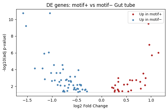
A volcano plot provides a quick overview of effect size (log2 fold change) vs significance.

import matplotlib.pyplot as plt

fig, ax = plt.subplots(figsize=(6, 4))

de = de_result.copy()
de["-log10(adj-pval)"] = -np.log10(de["adj-pval"].clip(lower=1e-300))

ax.scatter(
    de["log2fc"], de["-log10(adj-pval)"],
    c="grey", s=10, alpha=0.5,
)

# Highlight significant genes
sig = de[de["adj-pval"] < 0.05]
up = sig[sig["de_in"] == "group1"]  # motif+
down = sig[sig["de_in"] == "group2"]  # motif-
ax.scatter(up["log2fc"], up["-log10(adj-pval)"], c="firebrick", s=12, label="Up in motif+")
ax.scatter(down["log2fc"], down["-log10(adj-pval)"], c="steelblue", s=12, label="Up in motif−")

ax.axhline(-np.log10(0.05), color="grey", linestyle="--", linewidth=0.5)
ax.set_xlabel("log2 Fold Change")
ax.set_ylabel("-log10(adj p-value)")
ax.set_title(f"DE genes: motif+ vs motif− {anchor_ct}")
ax.legend(fontsize=9)
plt.tight_layout()
plt.show()